sqrt eigenvalues trend plots
Kushal K Dey 3/31/2018 Here we plot the trends of the square root of the eigenvalues of the estimated correlation matrices using different approaches - CorShrink, glasso and corpcor - against the tru correlation matrix.
library(ggplot2)
library(gridExtra)
Simulation Scripts
We run the following scripts for different choices of \(n\) and \(p\) for the Hub, Toeplitz and Banded Precision matrices.
Hub
source("../code/Figure2/eigenvalues_distribution_hub.R")
Toeplitz
source("../code/Figure2/eigenvalues_distribution_toeplitz.R")
Banded Precision
source("../code/Figure2/eigenvalues_distribution_sparse_nonsparse.R")The outputs from running each of these are saved under /shared_output/eigenvalues_sqrt_distribution/ and are read as follows to perform the visualization.
Visualization
hub_sqrt_eigenvalues <- get(load("../shared_output/eigenvalues_sqrt_distribution/hub_sqrt_eigenvalues_distribution.rda"))
banded_prec_sqrt_eigenvalues <- get(load("../shared_output/eigenvalues_sqrt_distribution/banded_precision_sqrt_eigenvalues_distribution.rda"))
toeplitz_sqrt_eigenvalues <- get(load("../shared_output/eigenvalues_sqrt_distribution/toeplitz_sqrt_eigenvalues_distribution.rda"))
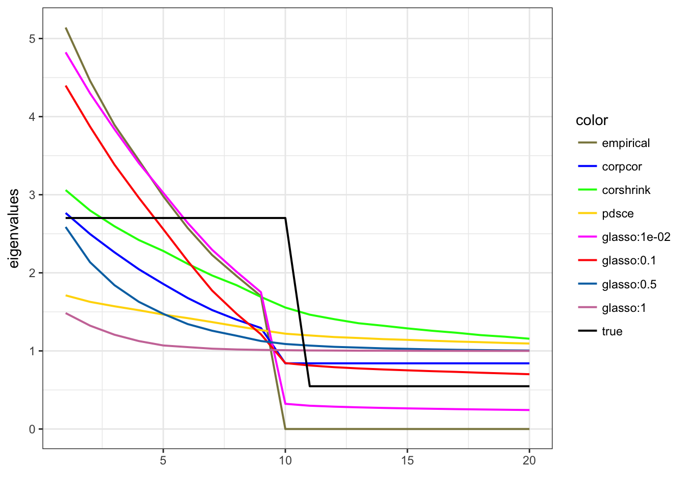
Example
eigenvalue_trends <- hub_sqrt_eigenvalues
num_samp <- c(30, 50, 100, 1000)
num <- 20
eigs.df <- data.frame ("x" = rep(1:num, 9),
                         "y" = eigenvalue_trends[[1]]$mean,
                         "color" = factor(c(rep("empirical", num),
                                     rep("corpcor",  num),
                                     rep("corshrink", num),
                                     rep("pdsce", num),
                                     rep("glasso:1e-02", num),
                                     rep("glasso:0.1", num),
                                     rep("glasso:0.5", num),
                                     rep("glasso:1", num),
                                     rep("true", num)), levels = c("empirical", "corpcor",
                                        "corshrink", "pdsce",
                                        "glasso:1e-02",
                                        "glasso:0.1",
                                        "glasso:0.5",
                                        "glasso:1", "true")),
                         "type" = c(rep("A", 8*num), rep("B", num)))

ggplot(eigs.df, aes(x=x, y=y, colour=color, linetype = color)) + geom_line(lty = 1, lwd = 0.7) +
    scale_linetype_manual(values = c(rep("solid", 4), rep("dashed", 1))) +
    scale_colour_manual(values=c("khaki4", "blue", "green", "gold", "magenta",
                                 "red", "#0072B2", "#CC79A7", "#000000")) + xlab("") + ylab("eigenvalues") +
    theme_bw()
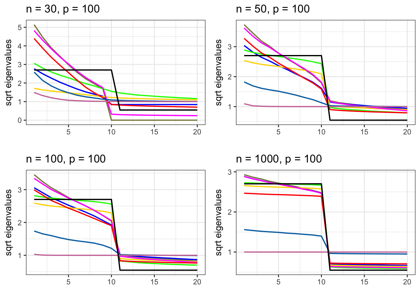
Plotting Hub sqrt eigenvalues
eigenvalue_trends <- hub_sqrt_eigenvalues
num_samp <- c(30, 50, 100, 1000)
num <- 20
gg <- list()
for(i in 1:4){
  eigs.df <- data.frame ("x" = rep(1:num, 9),
                         "y" = eigenvalue_trends[[i]]$mean,
                         "color" = factor(c(rep("empirical", num),
                                     rep("corpcor",  num),
                                     rep("corshrink", num),
                                     rep("pdsce", num),
                                     rep("glasso:1e-02", num),
                                     rep("glasso:0.1", num),
                                     rep("glasso:0.5", num),
                                     rep("glasso:1", num),
                                     rep("true", num)), levels = c("empirical", "corpcor",
                                        "corshrink", "pdsce",
                                        "glasso:1e-02",
                                        "glasso:0.1",
                                        "glasso:0.5",
                                        "glasso:1", "true")),
                         "type" = c(rep("A", 8*num), rep("B", num)))

 gg[[i]] <- ggplot(eigs.df, aes(x=x, y=y, colour=color, linetype = color)) +
                   geom_line(lty = 1, lwd = 0.7) +
                   scale_linetype_manual(values = c(rep("solid", 4), rep("dashed", 1))) +
                   scale_colour_manual(values=c("khaki4", "blue", "green", "gold", "magenta",
                                 "red", "#0072B2", "#CC79A7", "#000000")) + xlab("") +
                   ylab("sqrt eigenvalues") + ggtitle(paste0("n = ", num_samp[i], ", p = 100")) +
                   theme_bw() + theme(legend.position="none")
}

grid.arrange(gg[[1]], gg[[2]], gg[[3]],
             gg[[4]], nrow = 2, ncol = 2)
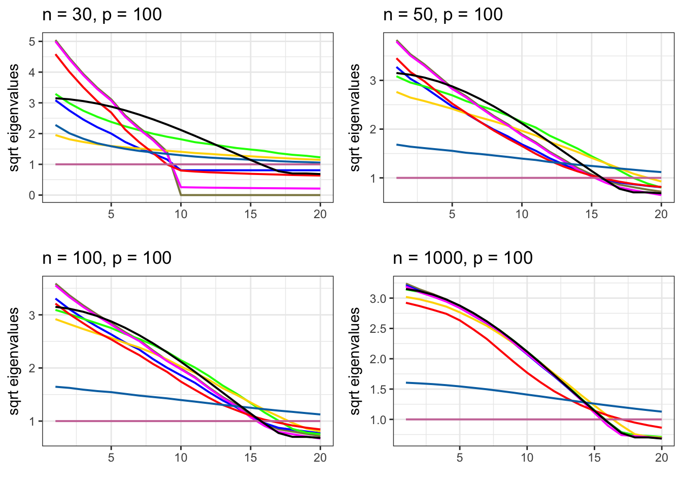
Plotting Toeplitz sqrt eigenvalues
eigenvalue_trends <- toeplitz_sqrt_eigenvalues
num_samp <- c(30, 50, 100, 1000)
num <- 20
for(i in 1:4){
  eigs.df <- data.frame ("x" = rep(1:num, 9),
                         "y" = eigenvalue_trends[[i]]$mean,
                         "color" = factor(c(rep("empirical", num),
                                     rep("corpcor",  num),
                                     rep("corshrink", num),
                                     rep("pdsce", num),
                                     rep("glasso:1e-02", num),
                                     rep("glasso:0.1", num),
                                     rep("glasso:0.5", num),
                                     rep("glasso:1", num),
                                     rep("true", num)), levels = c("empirical", "corpcor",
                                        "corshrink", "pdsce",
                                        "glasso:1e-02",
                                        "glasso:0.1",
                                        "glasso:0.5",
                                        "glasso:1", "true")),
                         "type" = c(rep("A", 8*num), rep("B", num)))

 gg[[(4+i)]] <- ggplot(eigs.df, aes(x=x, y=y, colour=color, linetype = color)) +
                   geom_line(lty = 1, lwd = 0.7) +
                   scale_linetype_manual(values = c(rep("solid", 4), rep("dashed", 1))) +
                   scale_colour_manual(values=c("khaki4", "blue", "green", "gold", "magenta",
                                 "red", "#0072B2", "#CC79A7", "#000000")) + xlab("") +
                   ylab("sqrt eigenvalues") + ggtitle(paste0("n = ", num_samp[i], ", p = 100")) +
                   theme_bw() + theme(legend.position="none")
}

grid.arrange(gg[[5]], gg[[6]], gg[[7]],
             gg[[8]], nrow = 2, ncol = 2)
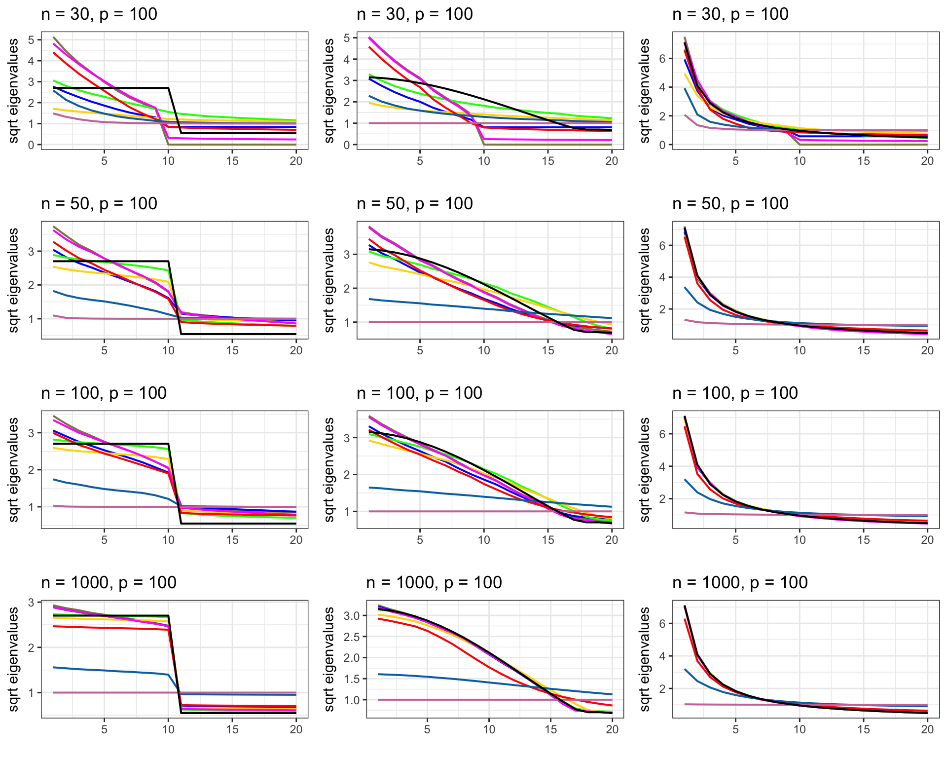
Plotting banded precision sqrt eigenvalues
eigenvalue_trends <- banded_prec_sqrt_eigenvalues
num_samp <- c(30, 50, 100, 1000)
num <- 20
for(i in 1:4){
  eigs.df <- data.frame ("x" = rep(1:num, 9),
                         "y" = eigenvalue_trends[[i]]$mean,
                         "color" = factor(c(rep("empirical", num),
                                     rep("corpcor",  num),
                                     rep("corshrink", num),
                                     rep("pdsce", num),
                                     rep("glasso:1e-02", num),
                                     rep("glasso:0.1", num),
                                     rep("glasso:0.5", num),
                                     rep("glasso:1", num),
                                     rep("true", num)), levels = c("empirical", "corpcor",
                                        "corshrink", "pdsce",
                                        "glasso:1e-02",
                                        "glasso:0.1",
                                        "glasso:0.5",
                                        "glasso:1", "true")),
                         "type" = c(rep("A", 8*num), rep("B", num)))

 gg[[(8+i)]] <- ggplot(eigs.df, aes(x=x, y=y, colour=color, linetype = color)) +
                   geom_line(lty = 1, lwd = 0.7) +
                   scale_linetype_manual(values = c(rep("solid", 4), rep("dashed", 1))) +
                   scale_colour_manual(values=c("khaki4", "blue", "green", "gold", "magenta",
                                 "red", "#0072B2", "#CC79A7", "#000000")) + xlab("") +
                   ylab("sqrt eigenvalues") + ggtitle(paste0("n = ", num_samp[i], ", p = 100")) +
                   theme_bw() + theme(legend.position="none")
}

grid.arrange(gg[[9]], gg[[10]], gg[[11]],
             gg[[12]], nrow = 2, ncol = 2)
grid.arrange(gg[[1]], gg[[2]], gg[[3]], gg[[4]],
             gg[[5]], gg[[6]], gg[[7]], gg[[8]],
             gg[[9]], gg[[10]], gg[[11]], gg[[12]],
             nrow = 4, ncol=3, as.table=FALSE)
This R Markdown site was created with workflowr