Illustration
We load an example data matrix - the person (544) by tissue samples (53) gene expression data for the gene ENSG00000166819 collected from the Genotype Tissue Expression (GTEx) Project .
data("sample_by_feature_data")Just by checking the first few rows and columns, we see that the data contains many missing values. The data is
sample_by_feature_data[1:5,1:5]## Adipose - Subcutaneous Adipose - Visceral (Omentum)
## GTEX-111CU 10.472332 10.84006
## GTEX-111FC 7.335392 NA
## GTEX-111VG 9.118889 NA
## GTEX-111YS 10.806459 11.26113
## GTEX-1122O 11.040446 11.71497
## Adrenal Gland Artery - Aorta Artery - Coronary
## GTEX-111CU 2.721234 NA NA
## GTEX-111FC NA NA NA
## GTEX-111VG NA NA NA
## GTEX-111YS 3.454823 1.162059 NA
## GTEX-1122O 1.522667 1.674467 4.188002CorShrinkData
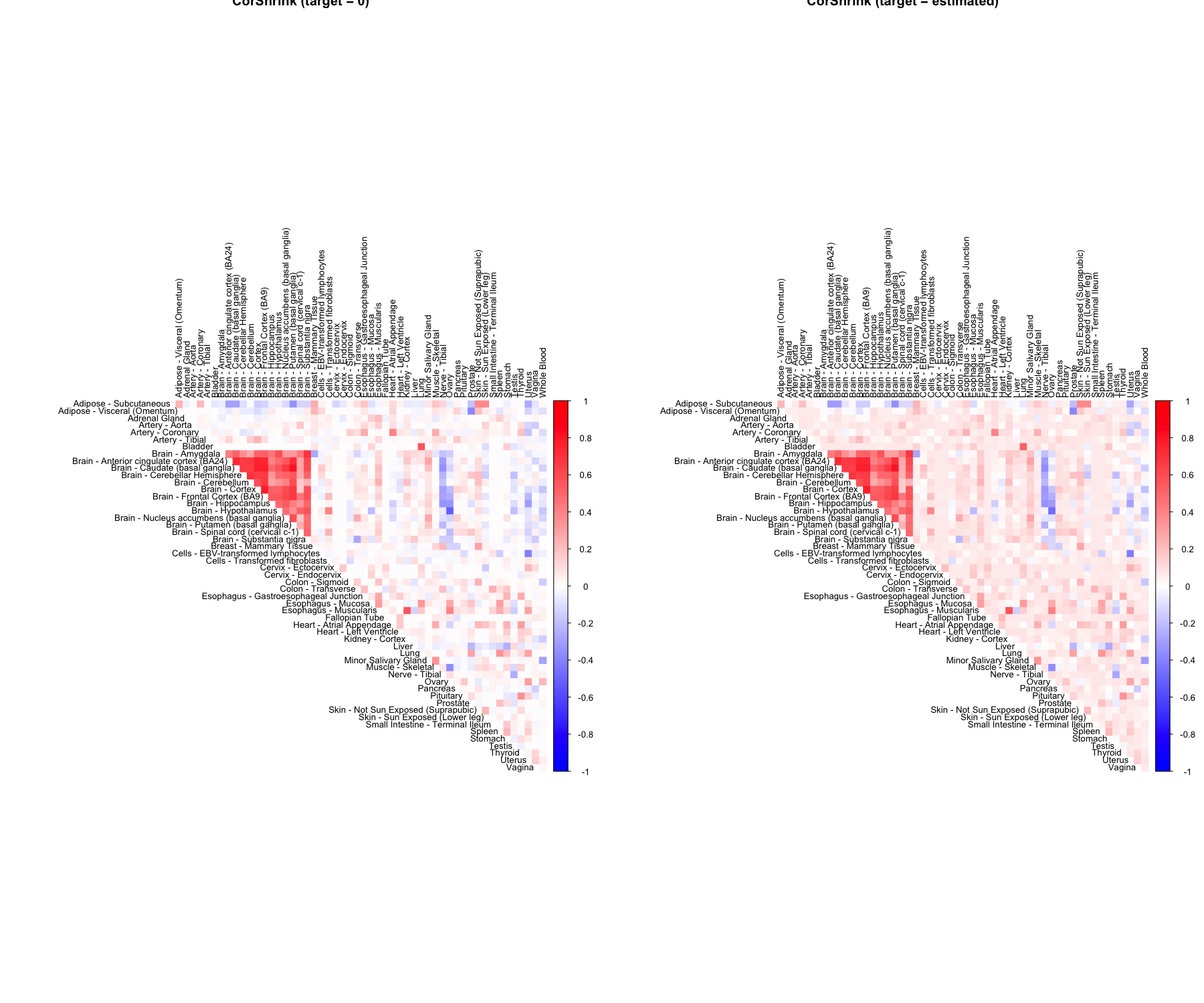
We estimate the adaptively shrunk correlation matrix for this data using CorShrink.
out <- CorShrinkData(sample_by_feature_data, sd_boot = FALSE, image = "both",
                     image.control = list(tl.cex = 0.8))
The function outputs a list with two elements which are two versions of CorShrink estimated matrices - cor and cor_before_PD.cor is the nearest positive definite approximation (\(R^{{\star}{\star}}\)) to cor_before_PD version (\(R^{{\star}}\)) as described in the methods above. When image = "both", the function plots the images for both these versions.
To see whether the method works well, check if the these two versions are close to each other.
out$cor_before_PD[1:5,1:5]## Adipose - Subcutaneous
## Adipose - Subcutaneous 1.00000000
## Adipose - Visceral (Omentum) 0.24093320
## Adrenal Gland -0.04403115
## Artery - Aorta 0.01330864
## Artery - Coronary 0.21663196
## Adipose - Visceral (Omentum) Adrenal Gland
## Adipose - Subcutaneous 0.240933205 -0.044031146
## Adipose - Visceral (Omentum) 1.000000000 0.002121612
## Adrenal Gland 0.002121612 1.000000000
## Artery - Aorta 0.004465918 -0.001097126
## Artery - Coronary 0.012401533 0.038526770
## Artery - Aorta Artery - Coronary
## Adipose - Subcutaneous 0.013308642 0.21663196
## Adipose - Visceral (Omentum) 0.004465918 0.01240153
## Adrenal Gland -0.001097126 0.03852677
## Artery - Aorta 1.000000000 0.03898770
## Artery - Coronary 0.038987702 1.00000000out$cor[1:5, 1:5]## Adipose - Subcutaneous
## Adipose - Subcutaneous 1.00000000
## Adipose - Visceral (Omentum) 0.24033223
## Adrenal Gland -0.04214076
## Artery - Aorta 0.01365631
## Artery - Coronary 0.21484578
## Adipose - Visceral (Omentum) Adrenal Gland
## Adipose - Subcutaneous 0.239003917 -0.0418844246
## Adipose - Visceral (Omentum) 1.000000000 0.0017177172
## Adrenal Gland 0.001718678 1.0000000000
## Artery - Aorta 0.003293150 -0.0008103749
## Artery - Coronary 0.013509246 0.0377365197
## Artery - Aorta Artery - Coronary
## Adipose - Subcutaneous 0.0135859012 0.21371816
## Adipose - Visceral (Omentum) 0.0032943783 0.01351303
## Adrenal Gland -0.0008111305 0.03776819
## Artery - Aorta 1.0000000000 0.03858038
## Artery - Coronary 0.0385839706 1.00000000CorShrinkMatrix
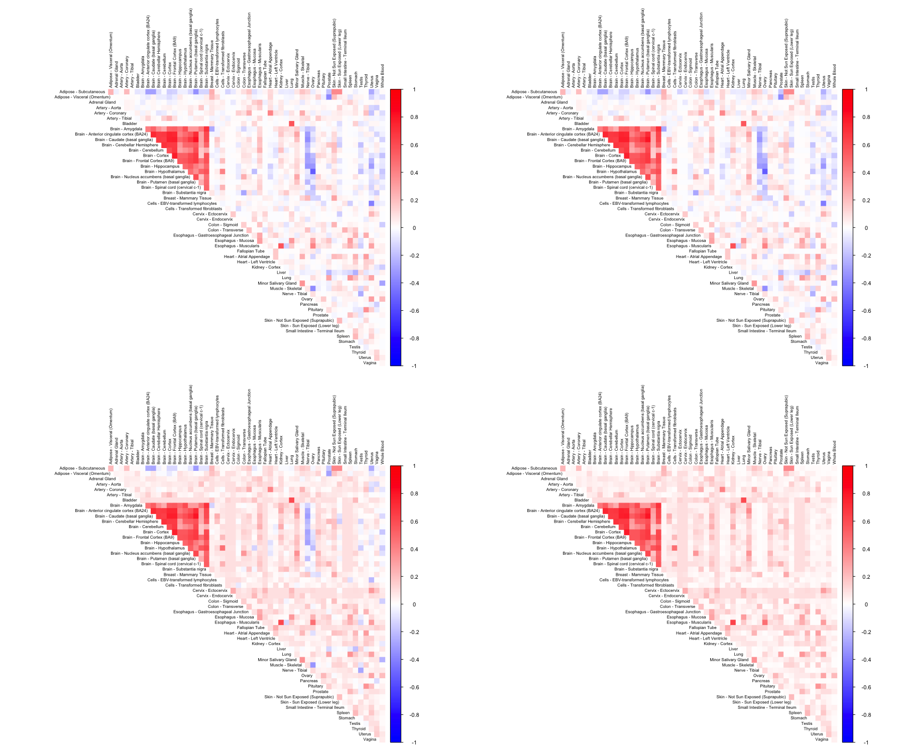
CorShrink takes as input not just the samples by features data matrix but also a matrix of pairwise correlations with a matrix of number of samples for each pair contributing to the correlation.
data("pairwise_corr_matrix")
data("common_samples")
out <- CorShrinkMatrix(pairwise_corr_matrix, common_samples, image = "both",
                       image.control = list(tl.cex = 0.8))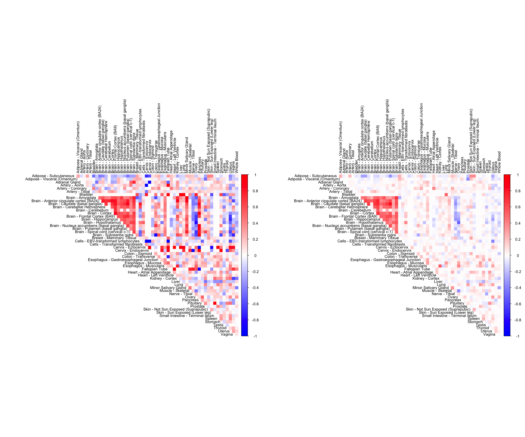
CorShrinkVector
CorShrink can be applied to vectors of correlations as well.
cor_vec <- c(-0.56, -0.4, 0.02, 0.2, 0.9, 0.8, 0.3, 0.1, 0.4)
nsamp_vec <- c(10, 20, 30, 4, 50, 60, 20, 10, 3)
out <- CorShrinkVector(corvec = cor_vec, nsamp_vec = nsamp_vec)
out
## [1] -0.1008065570 -0.0593108888 0.0006072387 0.0127953383 0.8944339076
## [6] 0.7935595323 0.0236537504 0.0051443096 0.0250218532Note that the correlations computed from adequate amount of data as for the 5th and 6th entries above, the amount of shrinkage is minimal, while it is substantial for the 4th and 9th entries which correspond to small number of samples.
CorShrinkData - resampling
We have so far looked at CorShrinkData, CorShrinkMatrix and CorShrinkVector, three functions that provide adaptive shrinkage of correlations at the level of the data matrix, matrix of correlations and vector of correlations respectively. In the above examples, we have used the asymptotic version of our algorithm (see Methods). Next we show example usage of a resampling based version of CorShrink.
out <- CorShrinkData(sample_by_feature_data, sd_boot = TRUE, image = "both",
                     image.control = list(tl.cex = 0.8))
## Finished Bootstrap : 1
## Finished Bootstrap : 2
## Finished Bootstrap : 3
## Finished Bootstrap : 4
## Finished Bootstrap : 5
## Finished Bootstrap : 6
## Finished Bootstrap : 7
## Finished Bootstrap : 8
## Finished Bootstrap : 9
## Finished Bootstrap : 10
## Finished Bootstrap : 11
## Finished Bootstrap : 12
## Finished Bootstrap : 13
## Finished Bootstrap : 14
## Finished Bootstrap : 15
## Finished Bootstrap : 16
## Finished Bootstrap : 17
## Finished Bootstrap : 18
## Finished Bootstrap : 19
## Finished Bootstrap : 20
## Finished Bootstrap : 21
## Finished Bootstrap : 22
## Finished Bootstrap : 23
## Finished Bootstrap : 24
## Finished Bootstrap : 25
## Finished Bootstrap : 26
## Finished Bootstrap : 27
## Finished Bootstrap : 28
## Finished Bootstrap : 29
## Finished Bootstrap : 30
## Finished Bootstrap : 31
## Finished Bootstrap : 32
## Finished Bootstrap : 33
## Finished Bootstrap : 34
## Finished Bootstrap : 35
## Finished Bootstrap : 36
## Finished Bootstrap : 37
## Finished Bootstrap : 38
## Finished Bootstrap : 39
## Finished Bootstrap : 40
## Finished Bootstrap : 41
## Finished Bootstrap : 42
## Finished Bootstrap : 43
## Finished Bootstrap : 44
## Finished Bootstrap : 45
## Finished Bootstrap : 46
## Finished Bootstrap : 47
## Finished Bootstrap : 48
## Finished Bootstrap : 49
## Finished Bootstrap : 50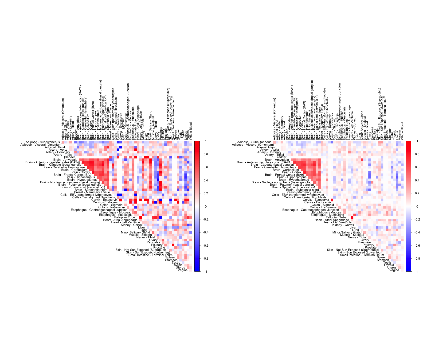
The algorithm works by first computing a Bootstrap estimate of the standard error of the Fisher z-scores for each pair and then using this estimate together with the correlations to shrink the latter.
CorShrinkMatrix - resampling
The breakdown can be formulated at the level of a correlation matrix as follows.
zscoreSDmat <- bootcorSE_calc(sample_by_feature_data, verbose = FALSE)
out <- CorShrinkMatrix(pairwise_corr_matrix, zscore_sd = zscoreSDmat, image = "both",
                       image.control = list(tl.cex = 0.8))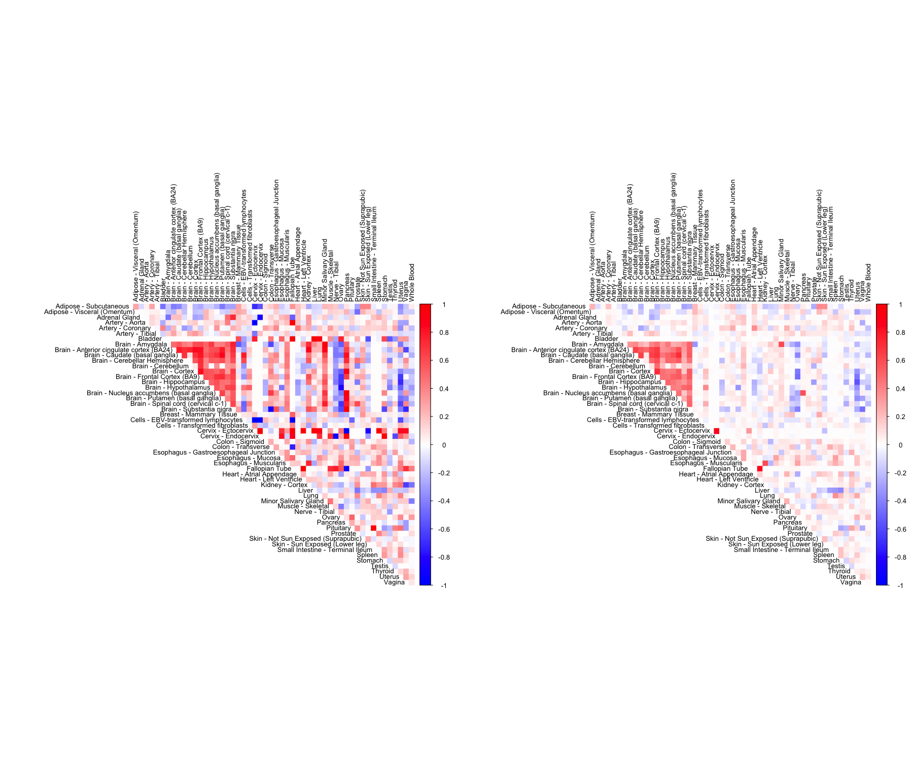
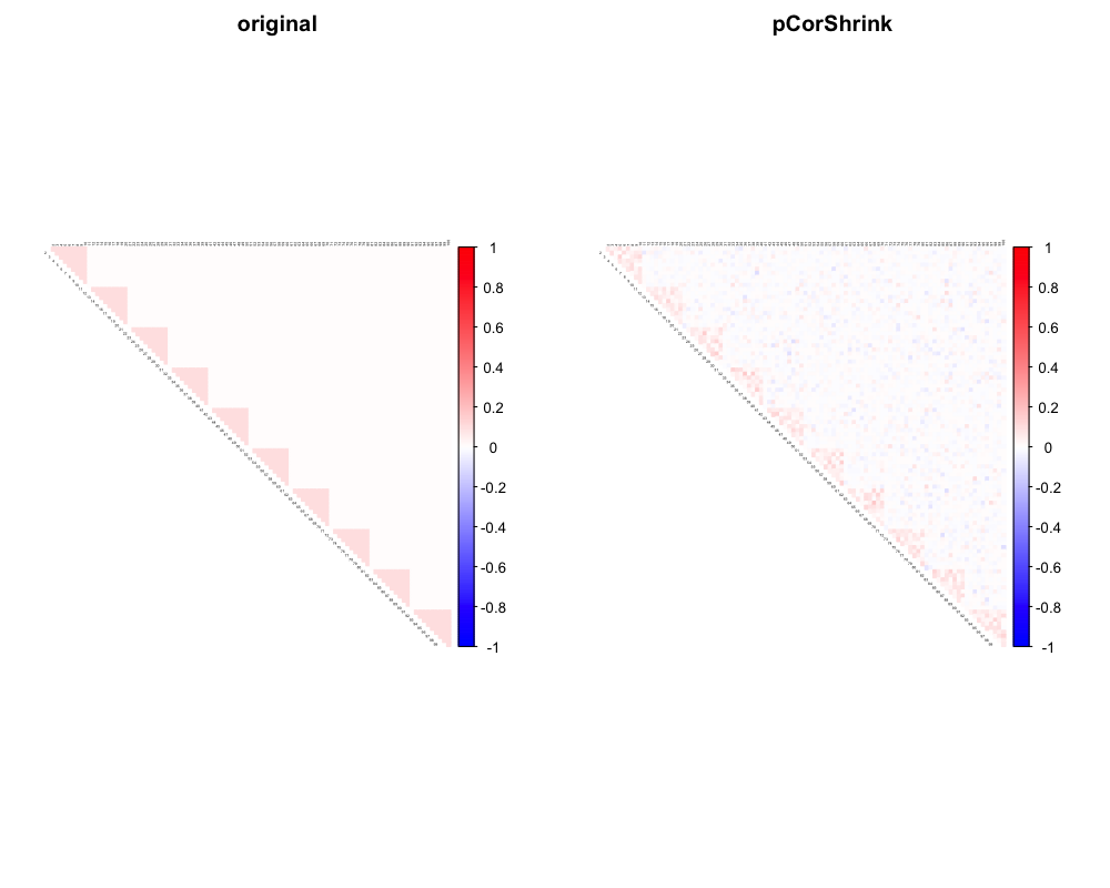
pCorShrink
We can use the pCorShrinkData function to adaptively shrink partial correlations. This approach is analogous to GLASSO, CLIME and other sparse graphical model methods, but pCorShrinkData shrinks the edge weights in the graph to 0 adaptively.
As per current implementation pCorShrinkData does not handle missing observations in the data matrix. So, we demonstrate the use of this method on a fully observed simulated data.
Simulated setting
library(Matrix)
n <- 500
P <- 100
block <- 10
mat <- 0.3*diag(1,block) + 0.7*rep(1,block) %*% t(rep(1, block))
Sigma <-   Matrix::bdiag(mat, mat, mat, mat, mat, mat, mat, mat, mat, mat)
corSigma <- cov2cor(Sigma)
pcorSigma <- corpcor::cor2pcor(corSigma)  ##  true partial correlation matrix
Generate Data
##################  Generate data   ################

data <- MASS::mvrnorm(n,rep(0,P),Sigma)
pCorShrinkData
out1 <- pCorShrinkData(data, reg_type = "lm")Visualization
library(corrplot)
col2 <- c("blue", "white", "red")
par(mfrow=c(1,2))
corrplot::corrplot(pcorSigma, diag = FALSE,
         col = colorRampPalette(col2)(200),
         tl.pos = "td", tl.cex = 0.2, tl.col = "black",
         rect.col = "white",na.label.col = "white", mar=c(2,2,2,2),
         method = "color", type = "upper", title = "original")
corrplot::corrplot(out1, diag = FALSE,
         col = colorRampPalette(col2)(200),
         tl.pos = "td", tl.cex = 0.2, tl.col = "black",
         rect.col = "white",na.label.col = "white", mar=c(2,2,2,2),
         method = "color", type = "upper", title = "pCorShrink")