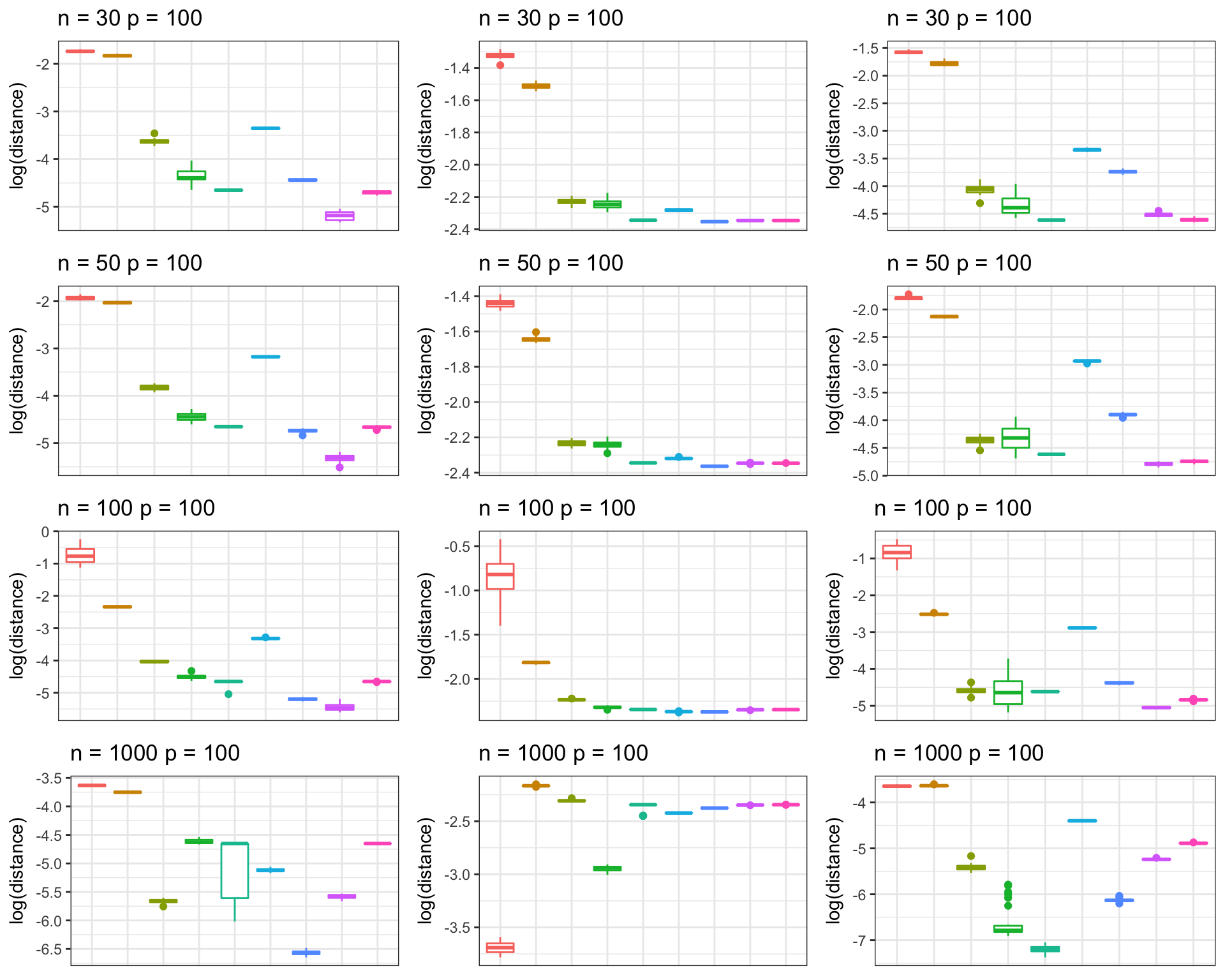
CLIME, pCorShrink and ISEE comparison
Kushal K Dey June 30, 2018 In this script, we compare the Frobenius norm distance of the estimated partial correlation matrices from CLIME, GLASSO, ISEE and pCorShrink approaches, with that of the original partial correlation matrix for different structural assumptions on the original correlation matrix.
Packages
library(MASS)
library(Matrix)
library(CorShrink)
library(corpcor)
library(glasso)
library(scio)
library(ggplot2)
library(scales)
library(gridExtra)
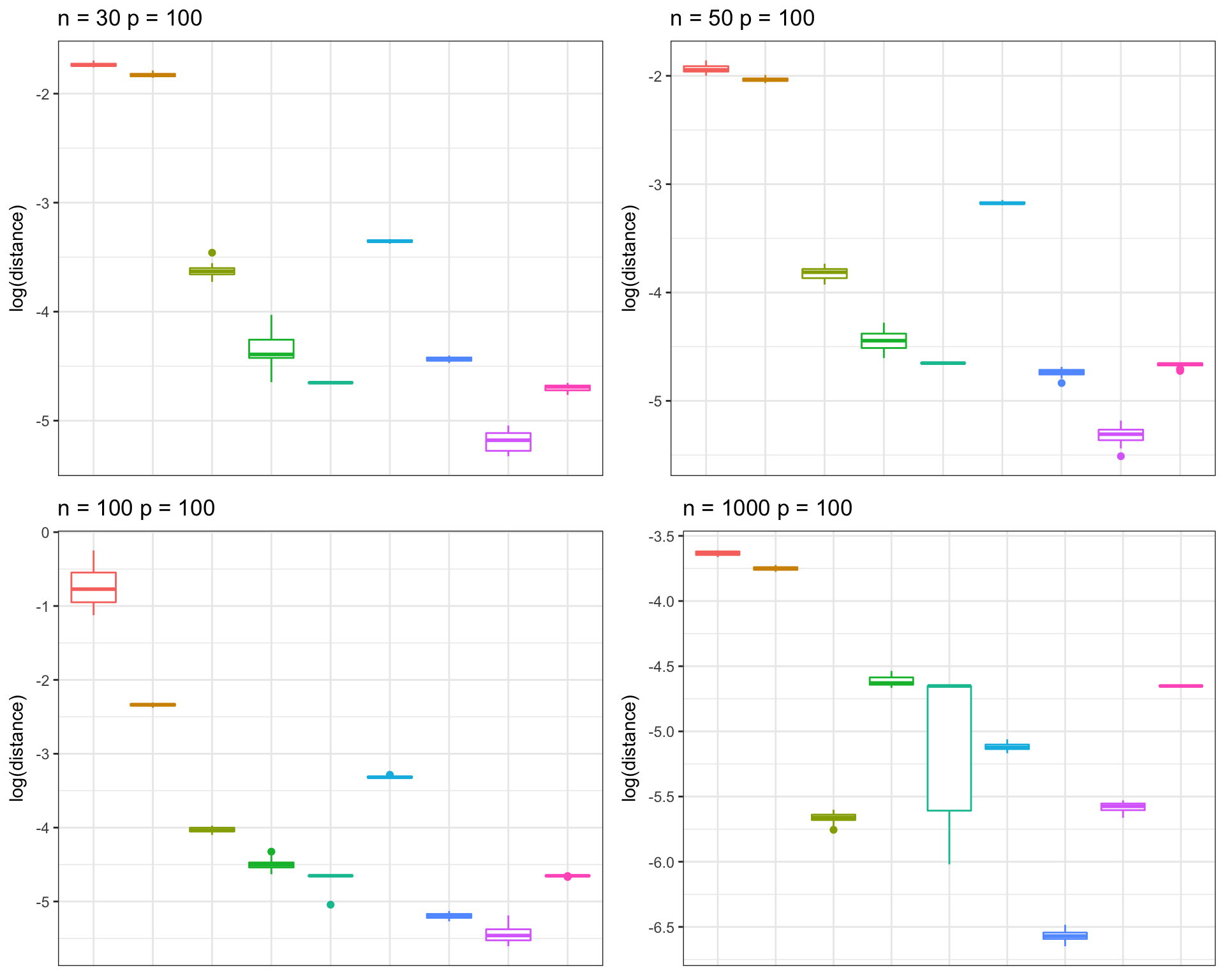
Hub correlation
frobs_list <- get(load("../shared_output/pcorshrink/frob_dist_hub.rda"))n_vec = c(30, 50, 100, 1000)
M = 30
p_list <- list()
for(n in 1:4){
df <- data.frame("method" = factor(c(rep("empirical", M), rep("isee_X", M),
rep("isee", M),
rep("pcorshrink_lasso", M),
rep("CLIME", M),
rep("glasso-0.01", M),
rep("glasso-0.1", M),
rep("glasso-0.5", M),
rep("glasso-1", M)),
levels = c("empirical", "isee_X",
"isee",
"pcorshrink_lasso",
"CLIME",
"glasso-0.01",
"glasso-0.1",
"glasso-0.5",
"glasso-1")),
"distance" = log(c(frobs_list$empirical[n,],
frobs_list$isee_X[n,],
frobs_list$isee[n,],
frobs_list$pcorshrink_lasso[n,],
frobs_list$clime[n,],
frobs_list$glasso_0_01[n,],
frobs_list$glasso_0_1[n,],
frobs_list$glasso_0_5[n,],
frobs_list$glasso_1[n,])))
p <- ggplot(df, aes(method, distance, color = method)) + ylab("log(distance)")
p_list[[n]] <- p + geom_boxplot() + theme_bw() + theme(legend.position = "none") +
theme(axis.title.x=element_blank(),
axis.text.x=element_blank(),
axis.ticks.x=element_blank()) + ggtitle(paste0("n = ", n_vec[n], " p = ", 100)) +scale_y_continuous(breaks= pretty_breaks())
}grid.arrange(p_list[[1]], p_list[[2]], p_list[[3]], p_list[[4]], nrow = 2, ncol=2, as.table=TRUE)
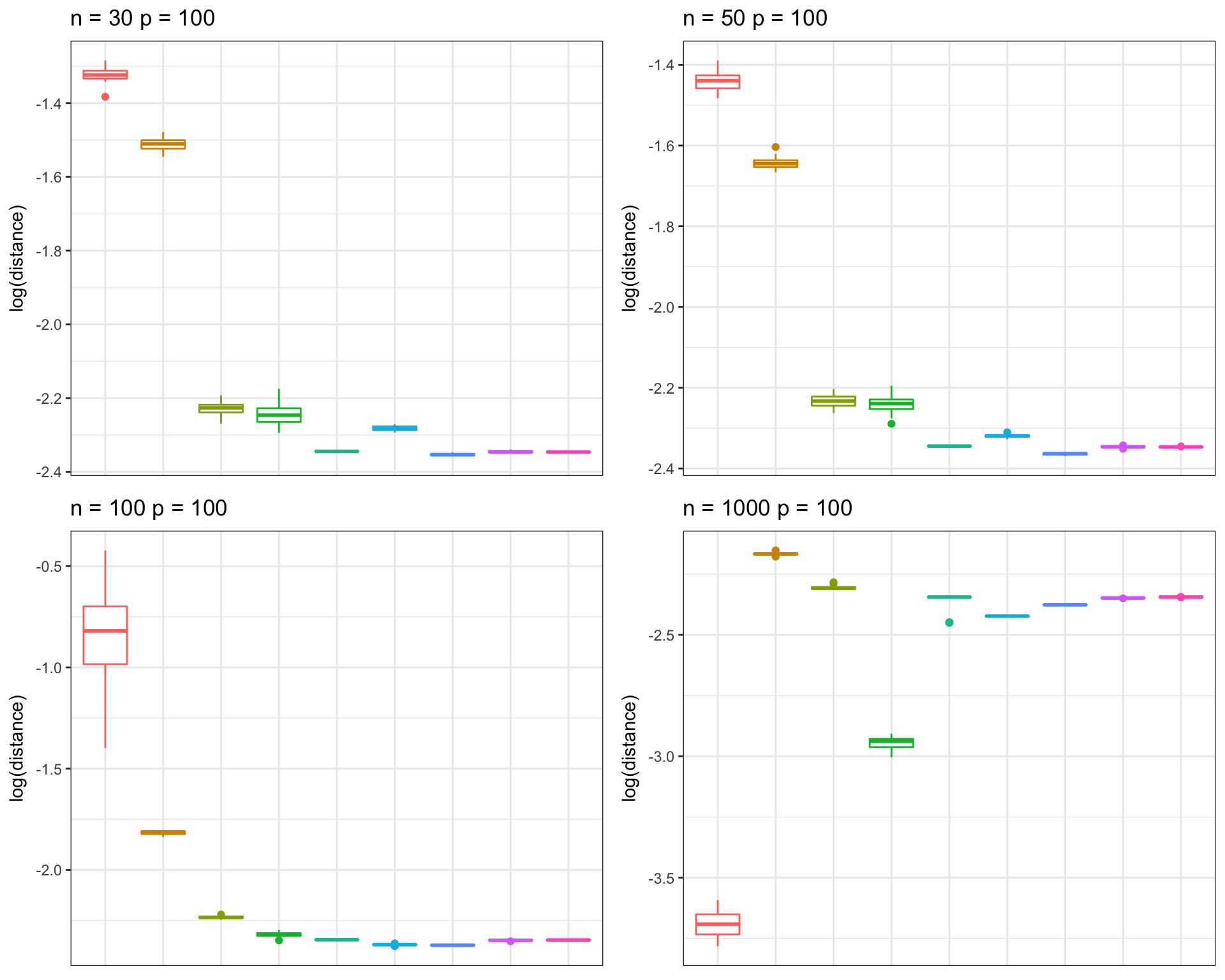
Toeplitz correlation
frobs_list <- get(load("../shared_output/pcorshrink/frob_dist_toeplitz.rda"))n_vec = c(30, 50, 100, 1000)
M = 30
for(n in 1:4){
df <- data.frame("method" = factor(c(rep("empirical", M), rep("isee_X", M),
rep("isee", M),
rep("pcorshrink_lasso", M),
rep("CLIME", M),
rep("glasso-0.01", M),
rep("glasso-0.1", M),
rep("glasso-0.5", M),
rep("glasso-1", M)),
levels = c("empirical", "isee_X",
"isee",
"pcorshrink_lasso",
"CLIME",
"glasso-0.01",
"glasso-0.1",
"glasso-0.5",
"glasso-1")),
"distance" = log(c(frobs_list$empirical[n,],
frobs_list$isee_X[n,],
frobs_list$isee[n,],
frobs_list$pcorshrink_lasso[n,],
frobs_list$clime[n,],
frobs_list$glasso_0_01[n,],
frobs_list$glasso_0_1[n,],
frobs_list$glasso_0_5[n,],
frobs_list$glasso_1[n,])))
p <- ggplot(df, aes(method, distance, color = method)) + ylab("log(distance)")
p_list[[(4+n)]] <- p + geom_boxplot() + theme_bw() + theme(legend.position = "none") +
theme(axis.title.x=element_blank(),
axis.text.x=element_blank(),
axis.ticks.x=element_blank()) + ggtitle(paste0("n = ", n_vec[n], " p = ", 100)) +scale_y_continuous(breaks= pretty_breaks())
}grid.arrange(p_list[[5]], p_list[[6]], p_list[[7]], p_list[[8]], nrow = 2, ncol=2, as.table=TRUE)
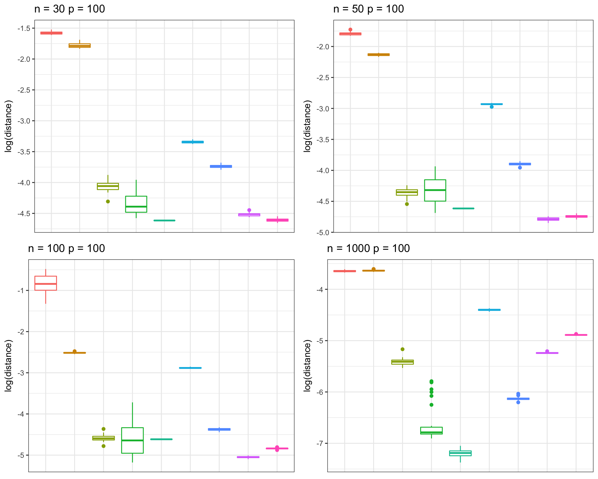
Banded Precision Matrix 1
frobs_list <- get(load("../shared_output/pcorshrink/frob_dist_banded_precision.rda"))n_vec = c(30, 50, 100, 1000)
M = 30
for(n in 1:4){
df <- data.frame("method" = factor(c(rep("empirical", M), rep("isee_X", M),
rep("isee", M),
rep("pcorshrink_lasso", M),
rep("CLIME", M),
rep("glasso-0.01", M),
rep("glasso-0.1", M),
rep("glasso-0.5", M),
rep("glasso-1", M)),
levels = c("empirical", "isee_X",
"isee",
"pcorshrink_lasso",
"CLIME",
"glasso-0.01",
"glasso-0.1",
"glasso-0.5",
"glasso-1")),
"distance" = log(c(frobs_list$empirical[n,],
frobs_list$isee_X[n,],
frobs_list$isee[n,],
frobs_list$pcorshrink_lasso[n,],
frobs_list$clime[n,],
frobs_list$glasso_0_01[n,],
frobs_list$glasso_0_1[n,],
frobs_list$glasso_0_5[n,],
frobs_list$glasso_1[n,])))
p <- ggplot(df, aes(method, distance, color = method)) + ylab("log(distance)")
p_list[[(8+n)]] <- p + geom_boxplot() + theme_bw() + theme(legend.position = "none") +
theme(axis.title.x=element_blank(),
axis.text.x=element_blank(),
axis.ticks.x=element_blank()) + ggtitle(paste0("n = ", n_vec[n], " p = ", 100)) +scale_y_continuous(breaks= pretty_breaks())
}grid.arrange(p_list[[9]], p_list[[10]], p_list[[11]], p_list[[12]], nrow = 2, ncol=2, as.table=TRUE)
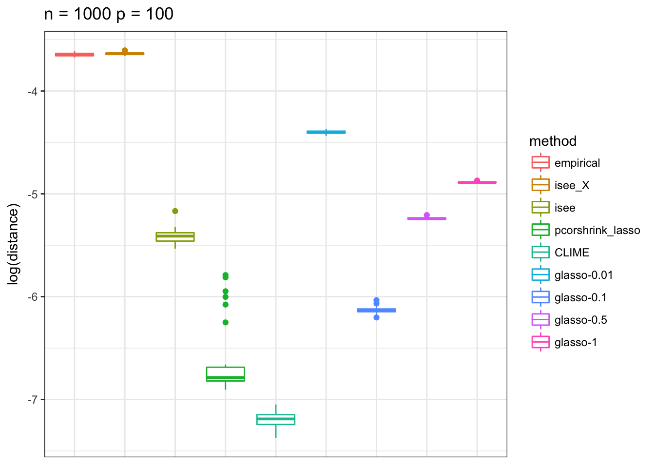
Banded Precision Matrix 2
p <- ggplot(df, aes(method, distance, color = method)) + ylab("log(distance)")
p + geom_boxplot() + theme_bw() +
  theme(axis.title.x=element_blank(),
        axis.text.x=element_blank(),
        axis.ticks.x=element_blank()) + ggtitle(paste0("n = ", n_vec[n], " p = ", 100)) +scale_y_continuous(breaks= pretty_breaks())
Aggregating all plots
grid.arrange(p_list[[1]], p_list[[2]], p_list[[3]], p_list[[4]],
             p_list[[5]], p_list[[6]], p_list[[7]], p_list[[8]],
             p_list[[9]], p_list[[10]], p_list[[11]], p_list[[12]],
             nrow = 4,  ncol=3, as.table = FALSE)
This R Markdown site was created with workflowr