Simulation Studies : Hub, Toeplitz correlation and Toeplitz precision
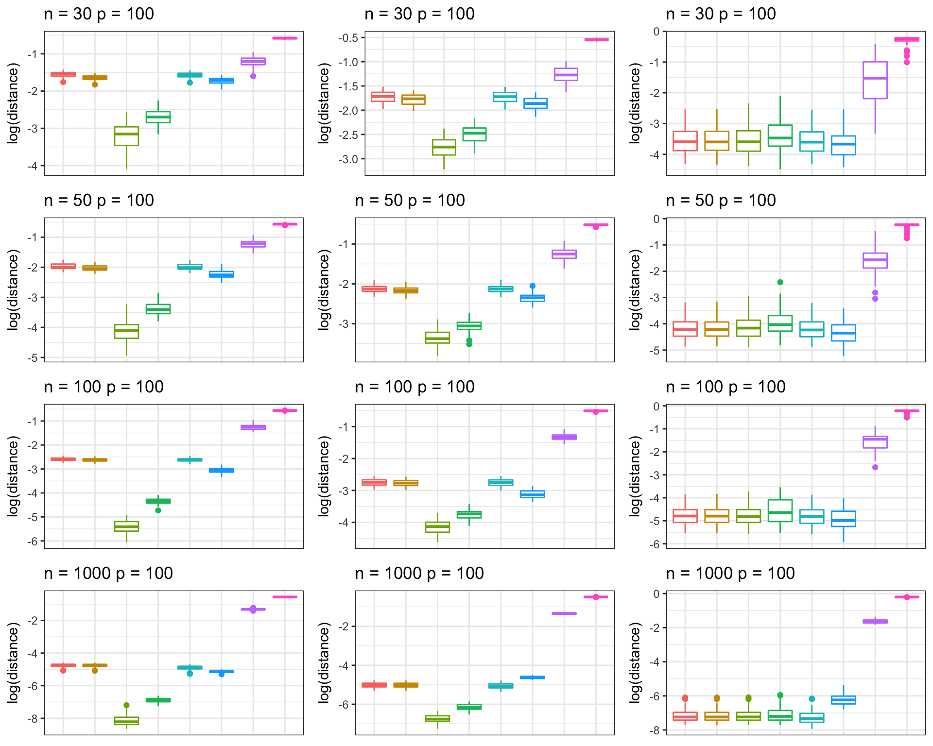
Kushal K Dey 2/23/2018 We perform box plot representation of the correlation matrix distance (CMD) between the population correlation matrix and correlation matrix estimators - CorShrink, Shafer Strimmer and the GLASSO methods.
Packages
library(gridExtra)
library(ggplot2)
library(scales)
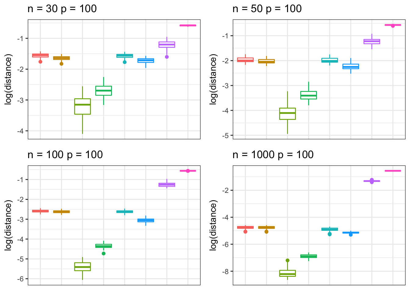
Hub correlation
We simulate data from a hub structured correlation matrix under different settings of \(n\) and \(p\) .
First run the code in
source("../code/Figure3/corshrink_hub.R")  ## n=50, p=100

## last line : save(frob_vals, file = paste0("hub_cmd_boot_n_", n, "_P_", P, "_results.rda"))
## change the file to the destination and file name you prefer.
Change the \(n\) and \(p\) accordingly, we pick \(p=100\) and vary \(n\) from \(30, 50, 100, 1000\) .
The final output from these files were saved under shared_output/CMD folders and can be read as follows.
hub_n_10_P_100 <- get(load("../shared_output/CMD/hub_cmd_boot_n_30_P_100_results.rda"))
hub_n_50_P_100 <- get(load("../shared_output/CMD/hub_cmd_boot_n_50_P_100_results.rda"))
hub_n_100_P_100 <- get(load("../shared_output/CMD/hub_cmd_boot_n_100_P_100_results.rda"))
hub_n_1000_P_100 <- get(load("../shared_output/CMD/hub_cmd_boot_n_1000_P_100_results.rda"))

df <- data.frame("method" = factor(c(rep("empirical", 50), rep("corpcor", 50), rep("corshrink", 50),
                              rep("pdsce",50), rep("glasso:1e-02", 50),
                              rep("glasso:0.1", 50), rep("glasso:0.5", 50), rep("glasso:1", 50)),
                              levels = c("empirical", "corpcor",
                                        "corshrink", "pdsce",
                                        "glasso:1e-02",
                                        "glasso:0.1",
                                        "glasso:0.5",
                                        "glasso:1")),
                 "distance" = log(c(hub_n_10_P_100[,1], hub_n_10_P_100[,2],
                                    hub_n_10_P_100[,3], hub_n_10_P_100[,4],
                                    hub_n_10_P_100[,5], hub_n_10_P_100[,6],
                                    hub_n_10_P_100[,7], hub_n_10_P_100[,8])))

p <- ggplot(df, aes(method, distance, color = method)) + ylab("log(distance)")
p1 <- p + geom_boxplot() + theme_bw() + theme(legend.position="none") +
  theme(axis.title.x=element_blank(),
        axis.text.x=element_blank(),
        axis.ticks.x=element_blank()) + ggtitle(paste0("n = ", 30, " p = ", 100)) +
scale_y_continuous(breaks= pretty_breaks())

df <- data.frame("method" = factor(c(rep("empirical", 50), rep("corpcor", 50), rep("corshrink", 50),
                              rep("pdsce",50), rep("glasso:1e-02", 50),
                              rep("glasso:0.1", 50), rep("glasso:0.5", 50), rep("glasso:1", 50)),
                              levels = c("empirical", "corpcor",
                                        "corshrink", "pdsce",
                                        "glasso:1e-02",
                                        "glasso:0.1",
                                        "glasso:0.5",
                                        "glasso:1")),
                 "distance" = log(c(hub_n_50_P_100[,1], hub_n_50_P_100[,2],
                                    hub_n_50_P_100[,3], hub_n_50_P_100[,4],
                                    hub_n_50_P_100[,5], hub_n_50_P_100[,6],
                                    hub_n_50_P_100[,7], hub_n_50_P_100[,8])))

p <- ggplot(df, aes(method, distance, color = method)) + ylab("log(distance)")
p2 <- p + geom_boxplot() + theme_bw() + theme(legend.position="none") +
  theme(axis.title.x=element_blank(),
        axis.text.x=element_blank(),
        axis.ticks.x=element_blank()) +  ggtitle(paste0("n = ", 50, " p = ", 100)) +
scale_y_continuous(breaks= pretty_breaks())


df <- data.frame("method" = factor(c(rep("empirical", 50), rep("corpcor", 50), rep("corshrink", 50),
                              rep("pdsce",50), rep("glasso:1e-02", 50),
                              rep("glasso:0.1", 50), rep("glasso:0.5", 50), rep("glasso:1", 50)),
                              levels = c("empirical", "corpcor",
                                        "corshrink", "pdsce",
                                        "glasso:1e-02",
                                        "glasso:0.1",
                                        "glasso:0.5",
                                        "glasso:1")),
                 "distance" = log(c(hub_n_100_P_100[,1], hub_n_100_P_100[,2],
                                    hub_n_100_P_100[,3], hub_n_100_P_100[,4],
                                    hub_n_100_P_100[,5], hub_n_100_P_100[,6],
                                    hub_n_100_P_100[,7], hub_n_100_P_100[,8]
                                    )))

p <- ggplot(df, aes(method, distance, color = method)) + ylab("log(distance)")
p3 <- p + geom_boxplot() + theme_bw() + theme(legend.position="none") +
  theme(axis.title.x=element_blank(),
        axis.text.x=element_blank(),
        axis.ticks.x=element_blank()) +  ggtitle(paste0("n = ", 100, " p = ", 100)) +
scale_y_continuous(breaks= pretty_breaks())

df <- data.frame("method" = factor(c(rep("empirical", 50), rep("corpcor", 50), rep("corshrink", 50),
                              rep("pdsce",50), rep("glasso:1e-02", 50),
                              rep("glasso:0.1", 50), rep("glasso:0.5", 50), rep("glasso:1", 50)),
                              levels = c("empirical", "corpcor",
                                        "corshrink", "pdsce",
                                        "glasso:1e-02",
                                        "glasso:0.1",
                                        "glasso:0.5",
                                        "glasso:1")),
                 "distance" = log(c(hub_n_1000_P_100[,1], hub_n_1000_P_100[,2],
                                    hub_n_1000_P_100[,3], hub_n_1000_P_100[,4],
                                    hub_n_1000_P_100[,5], hub_n_1000_P_100[,6],
                                    hub_n_1000_P_100[,7], hub_n_1000_P_100[,8]
                                    )))

p <- ggplot(df, aes(method, distance, color = method)) + ylab("log(distance)")
p4 <- p + geom_boxplot()+ theme_bw() + theme(legend.position="none") +
  theme(axis.title.x=element_blank(),
        axis.text.x=element_blank(),
        axis.ticks.x=element_blank()) + ggtitle(paste0("n = ", 1000, " p = ", 100)) +
scale_y_continuous(breaks= pretty_breaks())

grid.arrange(p1, p2, p3, p4, nrow = 2, ncol = 2)
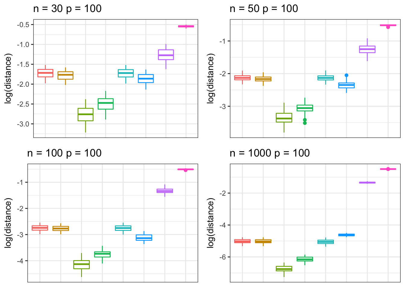
Toeplitz matrix
We simulate data from a Toeplitz structured correlation matrix under different settings of \(n\) and \(p\) .
First run the code in
source("../code/Figure3/corshrink_toeplitz.R")  ## n=50, p=100

## last line : save(frob_vals, file = paste0("toeplitz_cmd_boot_n_", n, "_P_", P, "_results.rda"))
## change the file to the destination and file name you prefer.
Change the \(n\) and \(p\) accordingly, we pick \(p=100\) and vary \(n\) from \(30, 50, 100, 1000\) .
The final output from these files were saved under shared_output/CMD folders and can be read as follows.
toeplitz_n_10_P_100 <- get(load("../shared_output/CMD/toeplitz_cmd_n_30_P_100_results.rda"))
toeplitz_n_50_P_100 <- get(load("../shared_output/CMD/toeplitz_cmd_n_50_P_100_results.rda"))
toeplitz_n_100_P_100 <- get(load("../shared_output/CMD/toeplitz_cmd_n_100_P_100_results.rda"))
toeplitz_n_1000_P_100 <- get(load("../shared_output/CMD/toeplitz_cmd_n_1000_P_100_results.rda"))

df <- data.frame("method" = factor(c(rep("empirical", 50), rep("corpcor", 50), rep("corshrink", 50),
                              rep("pdsce",50), rep("glasso:1e-02", 50),
                              rep("glasso:0.1", 50), rep("glasso:0.5", 50), rep("glasso:1", 50)),
                              levels = c("empirical", "corpcor",
                                        "corshrink", "pdsce",
                                        "glasso:1e-02",
                                        "glasso:0.1",
                                        "glasso:0.5",
                                        "glasso:1")),
                 "distance" = log(c(toeplitz_n_10_P_100[,1], toeplitz_n_10_P_100[,2],
                                    toeplitz_n_10_P_100[,3], toeplitz_n_10_P_100[,4],
                                    toeplitz_n_10_P_100[,5], toeplitz_n_10_P_100[,6],
                                    toeplitz_n_10_P_100[,7], toeplitz_n_10_P_100[,8])))

p <- ggplot(df, aes(method, distance, color = method)) + ylab("log(distance)")
p5 <- p + geom_boxplot() + theme_bw() + theme(legend.position="none") +
  theme(axis.title.x=element_blank(),
        axis.text.x=element_blank(),
        axis.ticks.x=element_blank()) + ggtitle(paste0("n = ", 30, " p = ", 100)) +
scale_y_continuous(breaks= pretty_breaks())

df <- data.frame("method" = factor(c(rep("empirical", 50), rep("corpcor", 50), rep("corshrink", 50),
                              rep("pdsce",50), rep("glasso:1e-02", 50),
                              rep("glasso:0.1", 50), rep("glasso:0.5", 50), rep("glasso:1", 50)),
                              levels = c("empirical", "corpcor",
                                        "corshrink", "pdsce",
                                        "glasso:1e-02",
                                        "glasso:0.1",
                                        "glasso:0.5",
                                        "glasso:1")),
                 "distance" = log(c(toeplitz_n_50_P_100[,1], toeplitz_n_50_P_100[,2],
                                    toeplitz_n_50_P_100[,3], toeplitz_n_50_P_100[,4],
                                    toeplitz_n_50_P_100[,5], toeplitz_n_50_P_100[,6],
                                    toeplitz_n_50_P_100[,7], toeplitz_n_50_P_100[,8])))

p <- ggplot(df, aes(method, distance, color = method)) + ylab("log(distance)")
p6 <- p + geom_boxplot() + theme_bw() + theme(legend.position="none") +
  theme(axis.title.x=element_blank(),
        axis.text.x=element_blank(),
        axis.ticks.x=element_blank()) +  ggtitle(paste0("n = ", 50, " p = ", 100)) +
scale_y_continuous(breaks= pretty_breaks())


df <- data.frame("method" = factor(c(rep("empirical", 50), rep("corpcor", 50), rep("corshrink", 50),
                              rep("pdsce",50), rep("glasso:1e-02", 50),
                              rep("glasso:0.1", 50), rep("glasso:0.5", 50), rep("glasso:1", 50)),
                              levels = c("empirical", "corpcor",
                                        "corshrink", "pdsce",
                                        "glasso:1e-02",
                                        "glasso:0.1",
                                        "glasso:0.5",
                                        "glasso:1")),
                 "distance" = log(c(toeplitz_n_100_P_100[,1], toeplitz_n_100_P_100[,2],
                                    toeplitz_n_100_P_100[,3], toeplitz_n_100_P_100[,4],
                                    toeplitz_n_100_P_100[,5], toeplitz_n_100_P_100[,6],
                                    toeplitz_n_100_P_100[,7], toeplitz_n_100_P_100[,8]
                                    )))

p <- ggplot(df, aes(method, distance, color = method)) + ylab("log(distance)")
p7 <- p + geom_boxplot() + theme_bw() + theme(legend.position="none") +
  theme(axis.title.x=element_blank(),
        axis.text.x=element_blank(),
        axis.ticks.x=element_blank()) +  ggtitle(paste0("n = ", 100, " p = ", 100)) +
scale_y_continuous(breaks= pretty_breaks())

df <- data.frame("method" = factor(c(rep("empirical", 50), rep("corpcor", 50), rep("corshrink", 50),
                              rep("pdsce",50), rep("glasso:1e-02", 50),
                              rep("glasso:0.1", 50), rep("glasso:0.5", 50), rep("glasso:1", 50)),
                              levels = c("empirical", "corpcor",
                                        "corshrink", "pdsce",
                                        "glasso:1e-02",
                                        "glasso:0.1",
                                        "glasso:0.5",
                                        "glasso:1")),
                 "distance" = log(c(toeplitz_n_1000_P_100[,1], toeplitz_n_1000_P_100[,2],
                                    toeplitz_n_1000_P_100[,3], toeplitz_n_1000_P_100[,4],
                                    toeplitz_n_1000_P_100[,5], toeplitz_n_1000_P_100[,6],
                                    toeplitz_n_1000_P_100[,7], toeplitz_n_1000_P_100[,8]
                                    )))

p <- ggplot(df, aes(method, distance, color = method)) + ylab("log(distance)")
p8 <- p + geom_boxplot()+ theme_bw() + theme(legend.position="none") +
  theme(axis.title.x=element_blank(),
        axis.text.x=element_blank(),
        axis.ticks.x=element_blank()) + ggtitle(paste0("n = ", 1000, " p = ", 100)) +
scale_y_continuous(breaks= pretty_breaks())

grid.arrange(p5, p6, p7, p8, nrow = 2, ncol = 2)
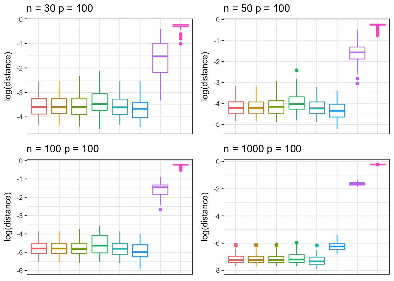
Banded precision matrix
We simulate data from a banded precision structured correlation matrix under different settings of \(n\) and \(p\) .
First run the code in
source("../code/Figure3/corshrink_banded_precision.R")  ## n=50, p=100

## last line : save(frob_vals, file = paste0("banded_precision_cmd_boot_n_", n, "_P_", P, "_results.rda"))
## change the file to the destination and file name you prefer.
Change the \(n\) and \(p\) accordingly, we pick \(p=100\) and vary \(n\) from \(30, 50, 100, 1000\) .
The final output from these files were ssaved under shared_output/CMD folders and can be read as follows.
banded_precision_n_10_P_100 <- get(load("../shared_output/CMD/banded_precision_n_30_P_100_results.rda"))
banded_precision_n_50_P_100 <- get(load("../shared_output/CMD/banded_precision_n_50_P_100_results.rda"))
banded_precision_n_100_P_100 <- get(load("../shared_output/CMD/banded_precision_n_100_P_100_results.rda"))
banded_precision_n_1000_P_100 <- get(load("../shared_output/CMD/banded_precision_n_1000_P_100_results.rda"))

df <- data.frame("method" = factor(c(rep("empirical", 50), rep("corpcor", 50), rep("corshrink", 50),
                              rep("pdsce",50), rep("glasso:1e-02", 50),
                              rep("glasso:0.1", 50), rep("glasso:0.5", 50), rep("glasso:1", 50)),
                              levels = c("empirical", "corpcor",
                                        "corshrink", "pdsce",
                                        "glasso:1e-02",
                                        "glasso:0.1",
                                        "glasso:0.5",
                                        "glasso:1")),
                 "distance" = log(c(banded_precision_n_10_P_100[,1], banded_precision_n_10_P_100[,2],
                                    banded_precision_n_10_P_100[,3], banded_precision_n_10_P_100[,4],
                                    banded_precision_n_10_P_100[,5], banded_precision_n_10_P_100[,6],
                                    banded_precision_n_10_P_100[,7], banded_precision_n_10_P_100[,8])))

p <- ggplot(df, aes(method, distance, color = method)) + ylab("log(distance)")
p9 <- p + geom_boxplot() + theme_bw() + theme(legend.position="none") +
  theme(axis.title.x=element_blank(),
        axis.text.x=element_blank(),
        axis.ticks.x=element_blank()) + ggtitle(paste0("n = ", 30, " p = ", 100)) +
scale_y_continuous(breaks= pretty_breaks())

df <- data.frame("method" = factor(c(rep("empirical", 50), rep("corpcor", 50), rep("corshrink", 50),
                              rep("pdsce",50), rep("glasso:1e-02", 50),
                              rep("glasso:0.1", 50), rep("glasso:0.5", 50), rep("glasso:1", 50)),
                              levels = c("empirical", "corpcor",
                                        "corshrink", "pdsce",
                                        "glasso:1e-02",
                                        "glasso:0.1",
                                        "glasso:0.5",
                                        "glasso:1")),
                 "distance" = log(c(banded_precision_n_50_P_100[,1], banded_precision_n_50_P_100[,2],
                                    banded_precision_n_50_P_100[,3], banded_precision_n_50_P_100[,4],
                                    banded_precision_n_50_P_100[,5], banded_precision_n_50_P_100[,6],
                                    banded_precision_n_50_P_100[,7], banded_precision_n_50_P_100[,8])))

p <- ggplot(df, aes(method, distance, color = method)) + ylab("log(distance)")
p10 <- p + geom_boxplot() + theme_bw() + theme(legend.position="none") +
  theme(axis.title.x=element_blank(),
        axis.text.x=element_blank(),
        axis.ticks.x=element_blank()) +  ggtitle(paste0("n = ", 50, " p = ", 100)) +
scale_y_continuous(breaks= pretty_breaks())


df <- data.frame("method" = factor(c(rep("empirical", 50), rep("corpcor", 50), rep("corshrink", 50),
                              rep("pdsce",50), rep("glasso:1e-02", 50),
                              rep("glasso:0.1", 50), rep("glasso:0.5", 50), rep("glasso:1", 50)),
                              levels = c("empirical", "corpcor",
                                        "corshrink", "pdsce",
                                        "glasso:1e-02",
                                        "glasso:0.1",
                                        "glasso:0.5",
                                        "glasso:1")),
                 "distance" = log(c(banded_precision_n_100_P_100[,1], banded_precision_n_100_P_100[,2],
                                    banded_precision_n_100_P_100[,3], banded_precision_n_100_P_100[,4],
                                    banded_precision_n_100_P_100[,5], banded_precision_n_100_P_100[,6],
                                    banded_precision_n_100_P_100[,7], banded_precision_n_100_P_100[,8]
                                    )))

p <- ggplot(df, aes(method, distance, color = method)) + ylab("log(distance)")
p11 <- p + geom_boxplot() + theme_bw() + theme(legend.position="none") +
  theme(axis.title.x=element_blank(),
        axis.text.x=element_blank(),
        axis.ticks.x=element_blank()) +  ggtitle(paste0("n = ", 100, " p = ", 100)) +
scale_y_continuous(breaks= pretty_breaks())

df <- data.frame("method" = factor(c(rep("empirical", 50), rep("corpcor", 50), rep("corshrink", 50),
                              rep("pdsce",50), rep("glasso:1e-02", 50),
                              rep("glasso:0.1", 50), rep("glasso:0.5", 50), rep("glasso:1", 50)),
                              levels = c("empirical", "corpcor",
                                        "corshrink", "pdsce",
                                        "glasso:1e-02",
                                        "glasso:0.1",
                                        "glasso:0.5",
                                        "glasso:1")),
                 "distance" = log(c(banded_precision_n_1000_P_100[,1], banded_precision_n_1000_P_100[,2],
                                    banded_precision_n_1000_P_100[,3], banded_precision_n_1000_P_100[,4],
                                    banded_precision_n_1000_P_100[,5], banded_precision_n_1000_P_100[,6],
                                    banded_precision_n_1000_P_100[,7], banded_precision_n_1000_P_100[,8]
                                    )))

p <- ggplot(df, aes(method, distance, color = method)) + ylab("log(distance)")
p12 <- p + geom_boxplot()+ theme_bw() + theme(legend.position="none") +
  theme(axis.title.x=element_blank(),
        axis.text.x=element_blank(),
        axis.ticks.x=element_blank()) + ggtitle(paste0("n = ", 1000, " p = ", 100)) +
scale_y_continuous(breaks= pretty_breaks())

grid.arrange(p9, p10, p11, p12, nrow = 2, ncol = 2)
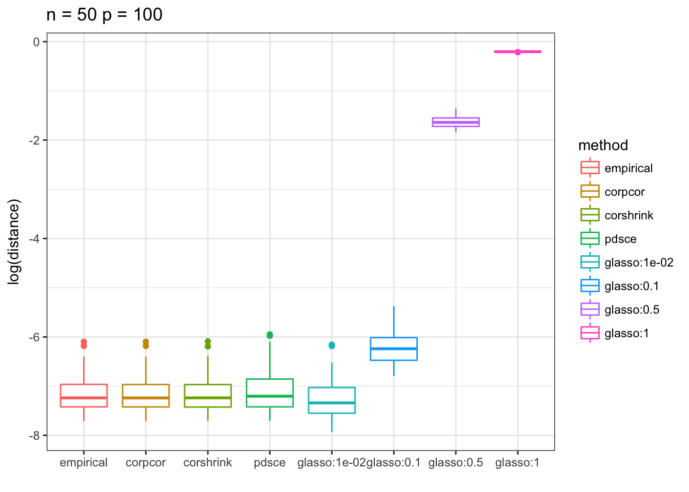
p <- ggplot(df, aes(method, distance, color = method)) + xlab("") + ylab("log(distance)")+ ggtitle("n=50, p = 100")
p13 <- p + geom_boxplot() + theme_bw() +
scale_y_continuous(breaks= pretty_breaks()) + ggtitle(paste0("n = ", 50, " p = ", 100))
print(p13)
grid.arrange(p1,p2,p3,p4,p5,p6,p7,p8,p9,p10,p11,p12, nrow = 4, ncol = 3, as.table = FALSE)
This R Markdown site was created with workflowr