Wallacea region GoM analysis : mammals and birds transpose
Kushal K Dey
6/8/2018
Intro
Here we observe the presence absence data of bird species in the Australasian region (Wallacea). We try to interpret that in the context of our Grade of Membership (GoM) model and its applications to presence absence data.
Packages
library(methClust)
library(CountClust)
library(rasterVis)
library(gtools)
library(sp)
library(rgdal)
library(ggplot2)
library(maps)
library(mapdata)
library(mapplots)
library(scales)
library(ggthemes)
Load the data
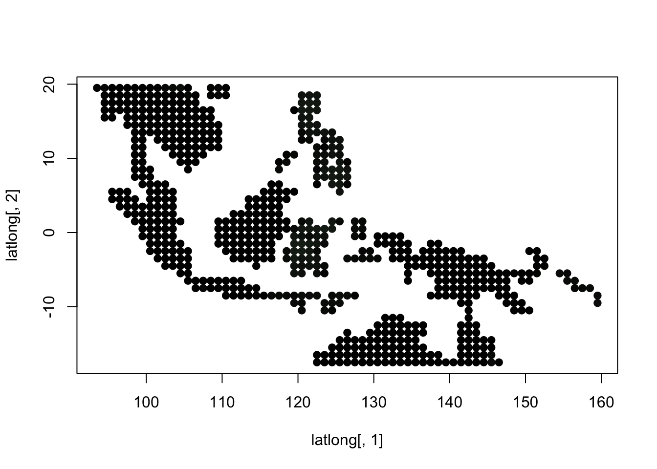
Wallacea Region data
birds <- get(load("../data/wallacea_mammals_birds.rda"))
latlong_chars_birds <- rownames(birds)
latlong <- cbind.data.frame(as.numeric(sapply(latlong_chars_birds,
              function(x) return(strsplit(x, "_")[[1]][1]))),
         as.numeric(sapply(latlong_chars_birds,
              function(x) return(strsplit(x, "_")[[1]][2]))))
Map of Wallacea
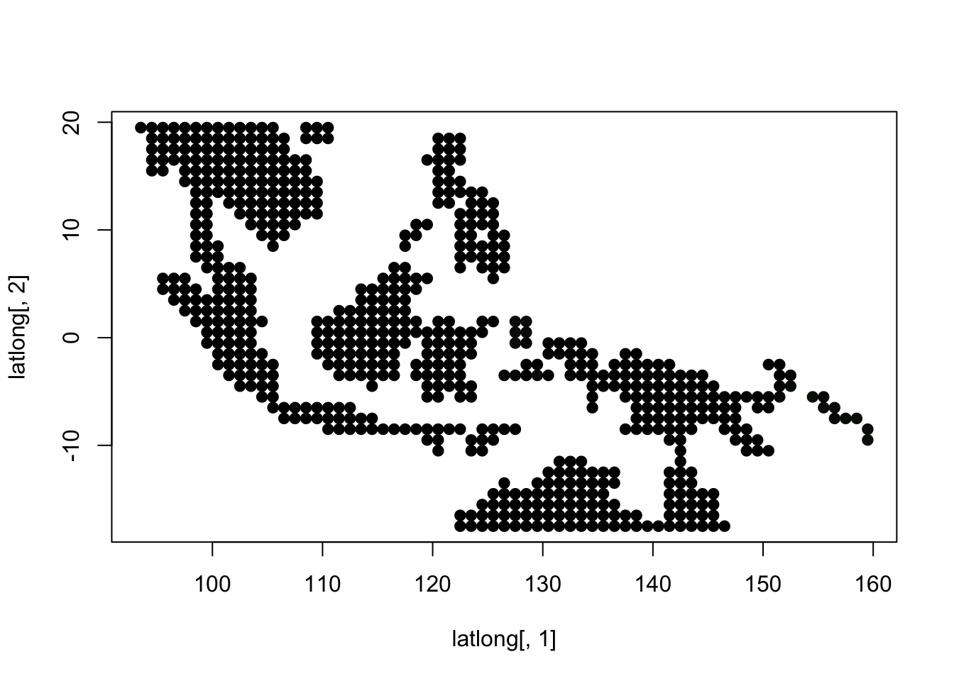
world_map <- map_data("world")
world_map <- world_map[world_map$region != "Antarctica",] # intercourse antarctica

world_map <- world_map[world_map$long > 90 & world_map$long < 160, ]
world_map <- world_map[world_map$lat > -18 & world_map$lat < 20, ]


p <- ggplot() + coord_fixed() +
  xlab("") + ylab("")

#Add map to base plot
base_world_messy <- p + geom_polygon(data=world_map, aes(x=long, y=lat, group=group), colour="light green", fill="light green")

cleanup <-
  theme(panel.grid.major = element_blank(), panel.grid.minor = element_blank(),
        panel.background = element_rect(fill = 'white', colour = 'white'),
        axis.line = element_line(colour = "white"), legend.position="none",
        axis.ticks=element_blank(), axis.text.x=element_blank(),
        axis.text.y=element_blank())

base_world <- base_world_messy + cleanup

base_world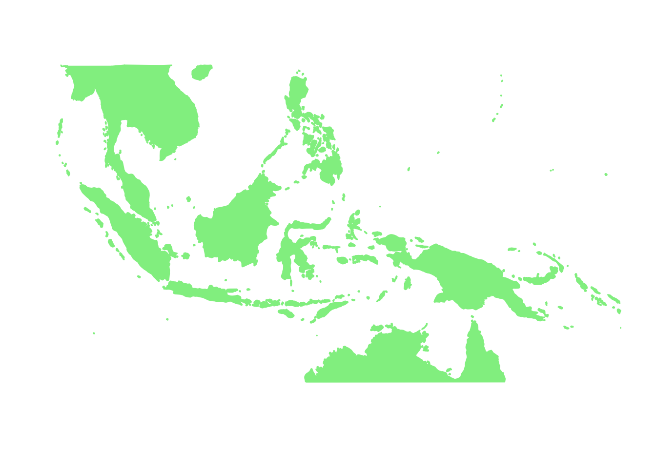
Visualization
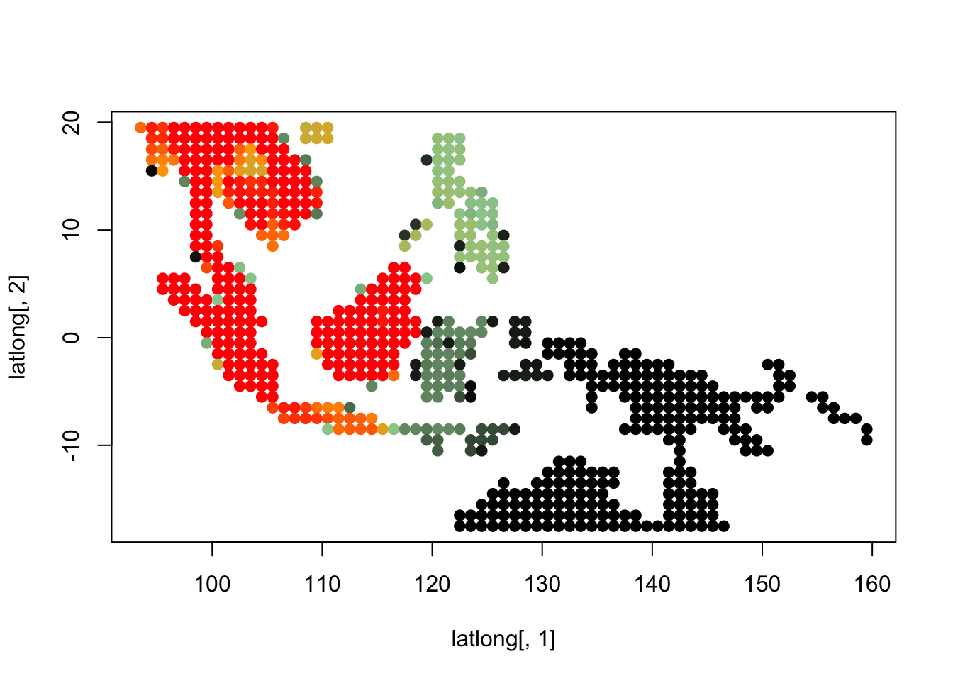
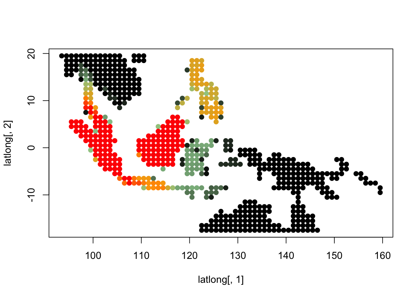
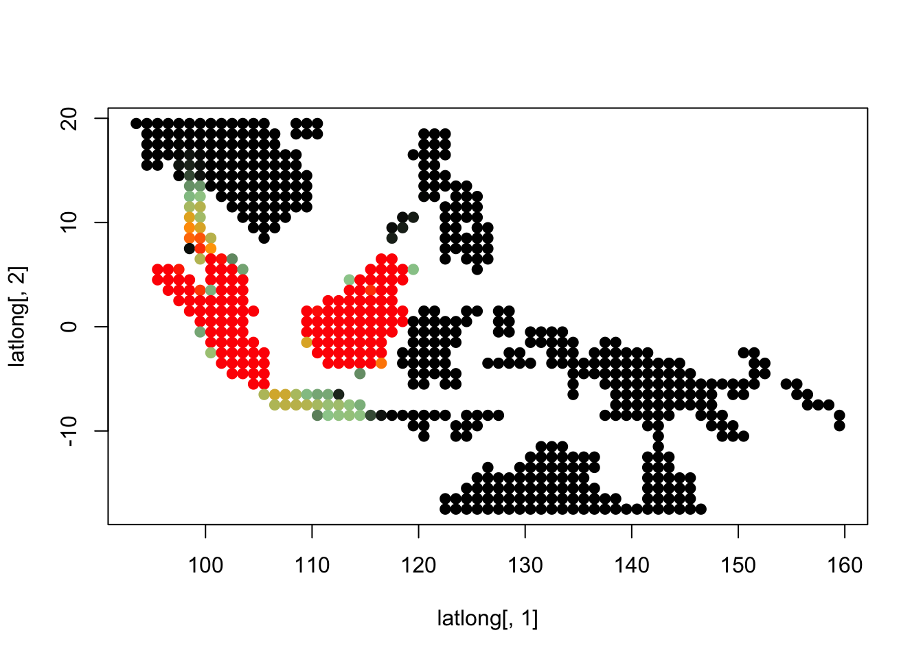
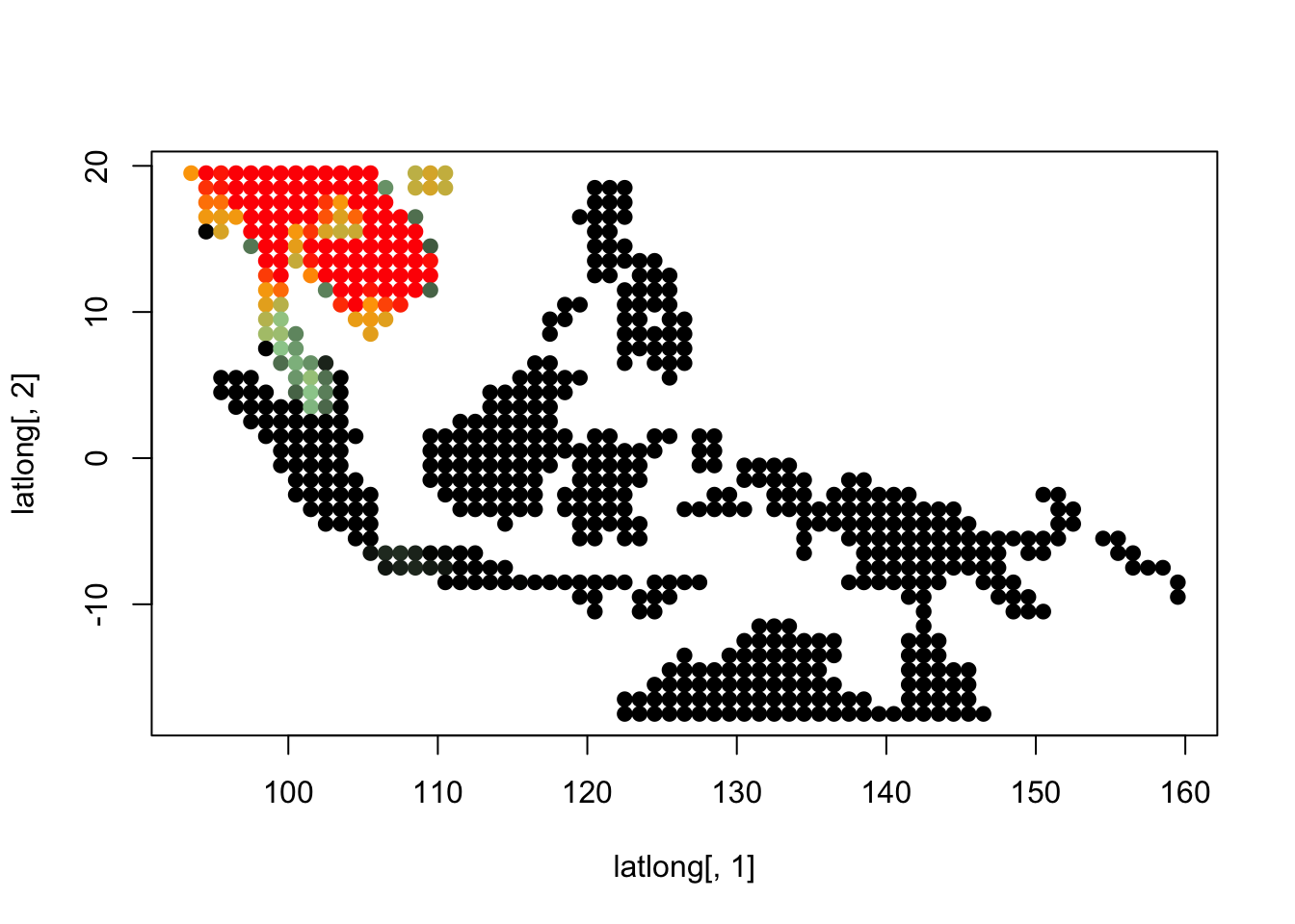
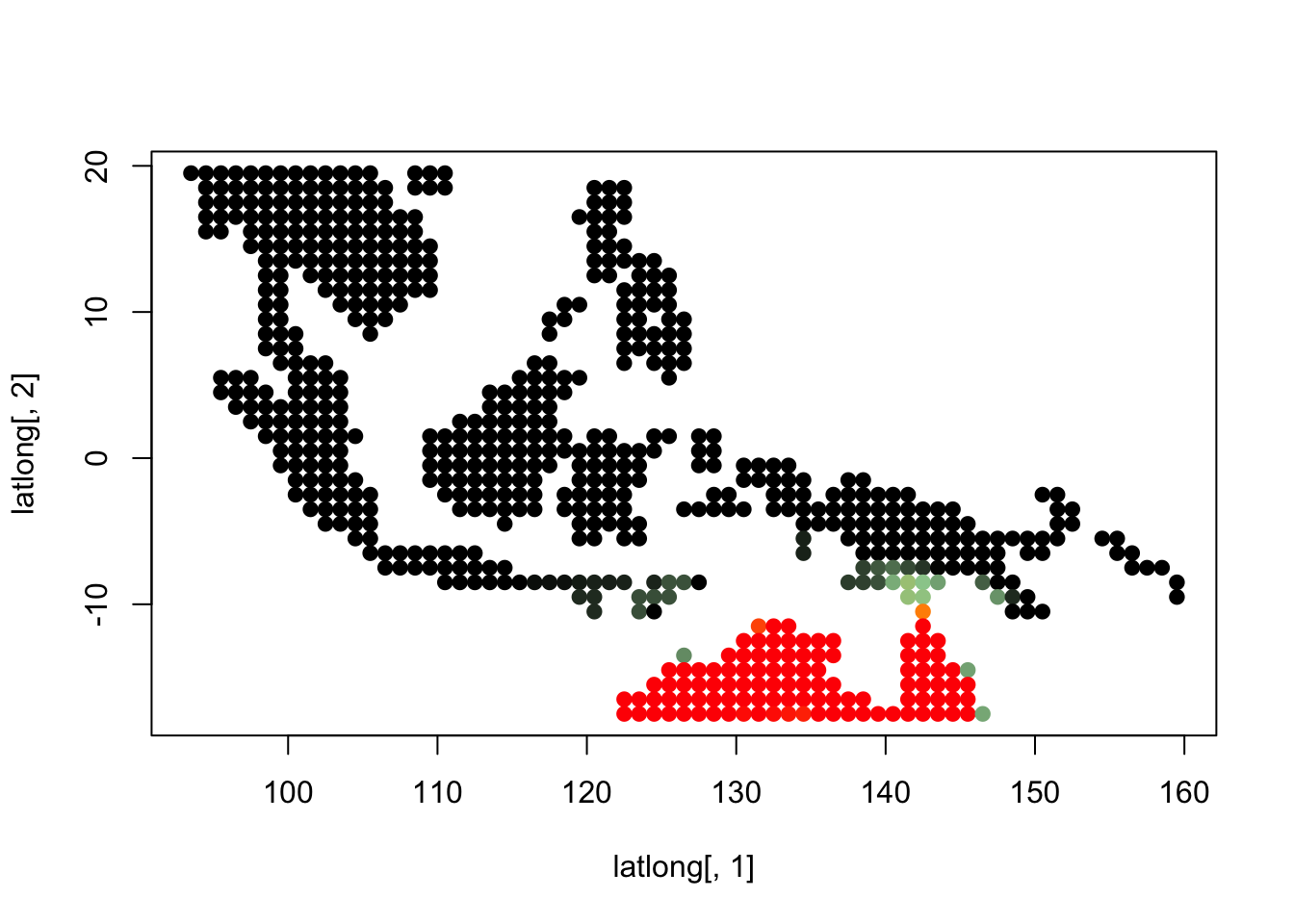
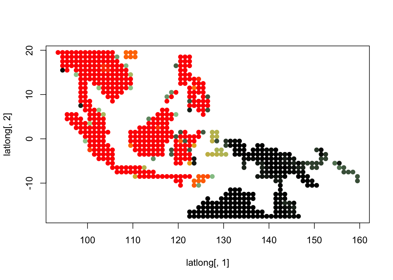
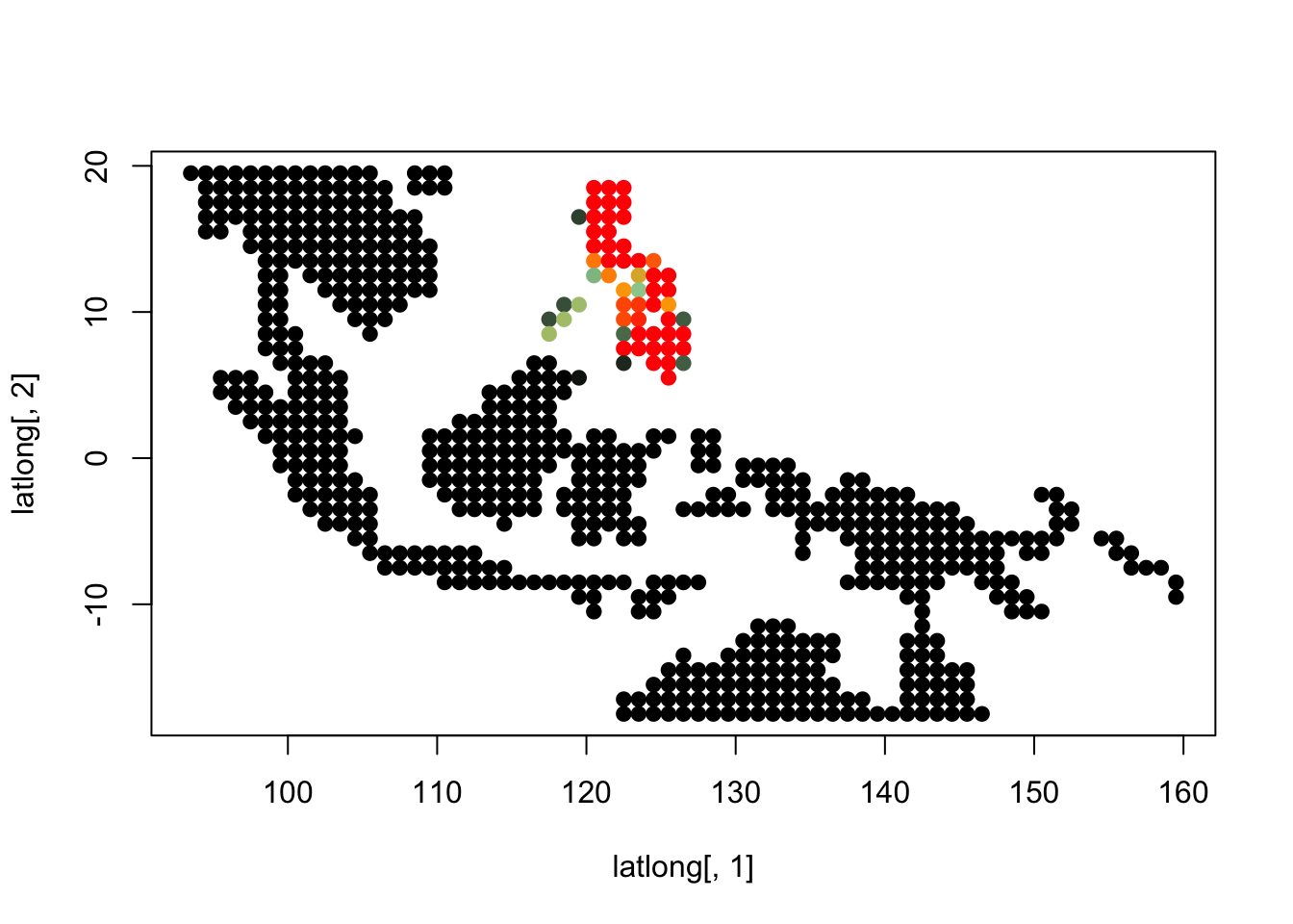
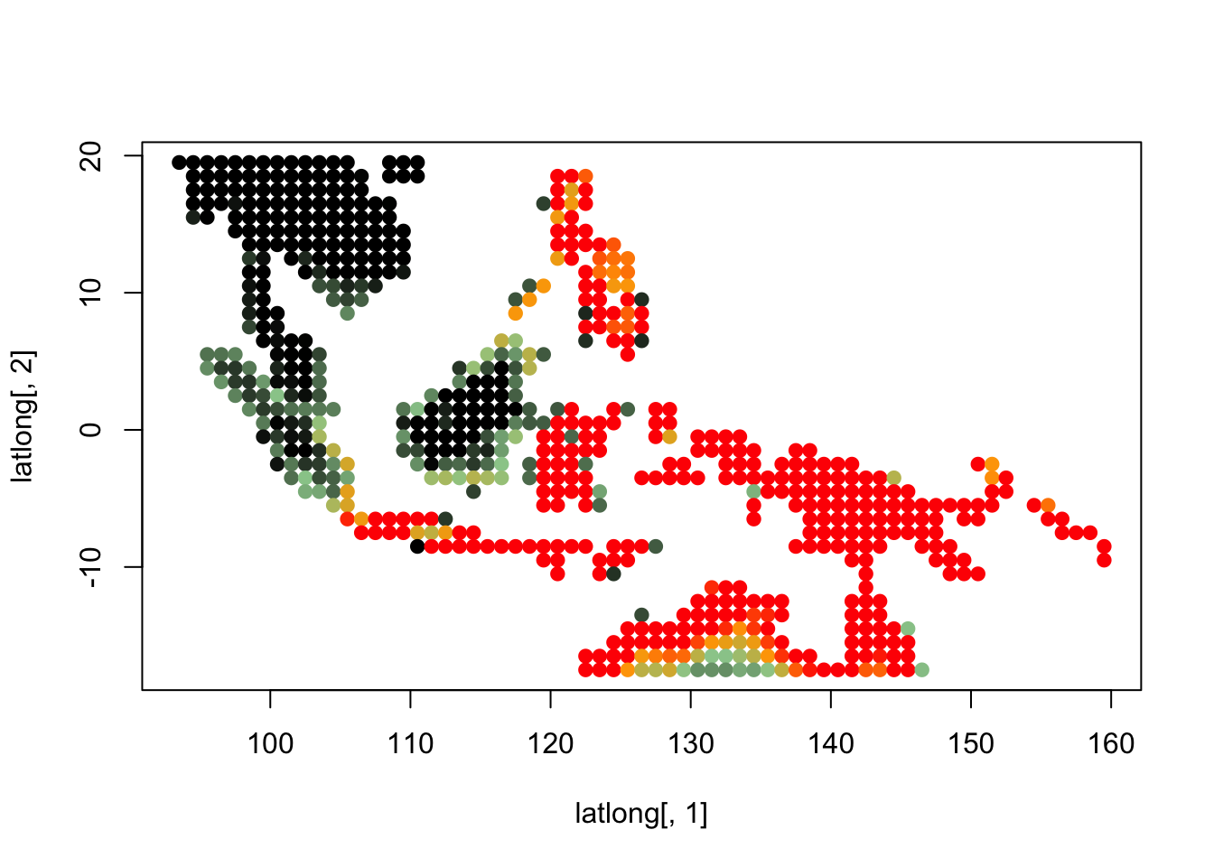
topics_clust <- get(load("../output/methClust_wallacea_mammals_and_birds_transpose.rda"))K = 3
topics <- topics_clust[[3]]
latlong_chars <- rownames(topics$freq)
latlong <- cbind.data.frame(as.numeric(sapply(latlong_chars,
              function(x) return(strsplit(x, "_")[[1]][1]))),
         as.numeric(sapply(latlong_chars,
              function(x) return(strsplit(x, "_")[[1]][2]))))

for(i in 1:dim(topics$freq)[2]){
  tmp <- round(1000*topics$freq[,i])+1
  colorGradient <- colorRampPalette(c("black", "darkseagreen3",
                                    "orange","red"))(1001)
  plot(latlong[,1], latlong[,2], col= colorGradient[tmp], pch = 20, cex = 1.5)
}
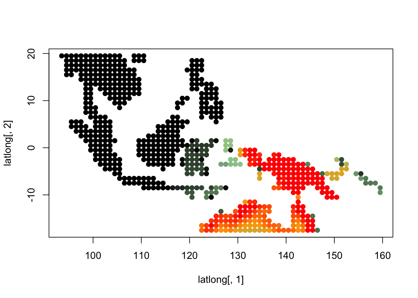
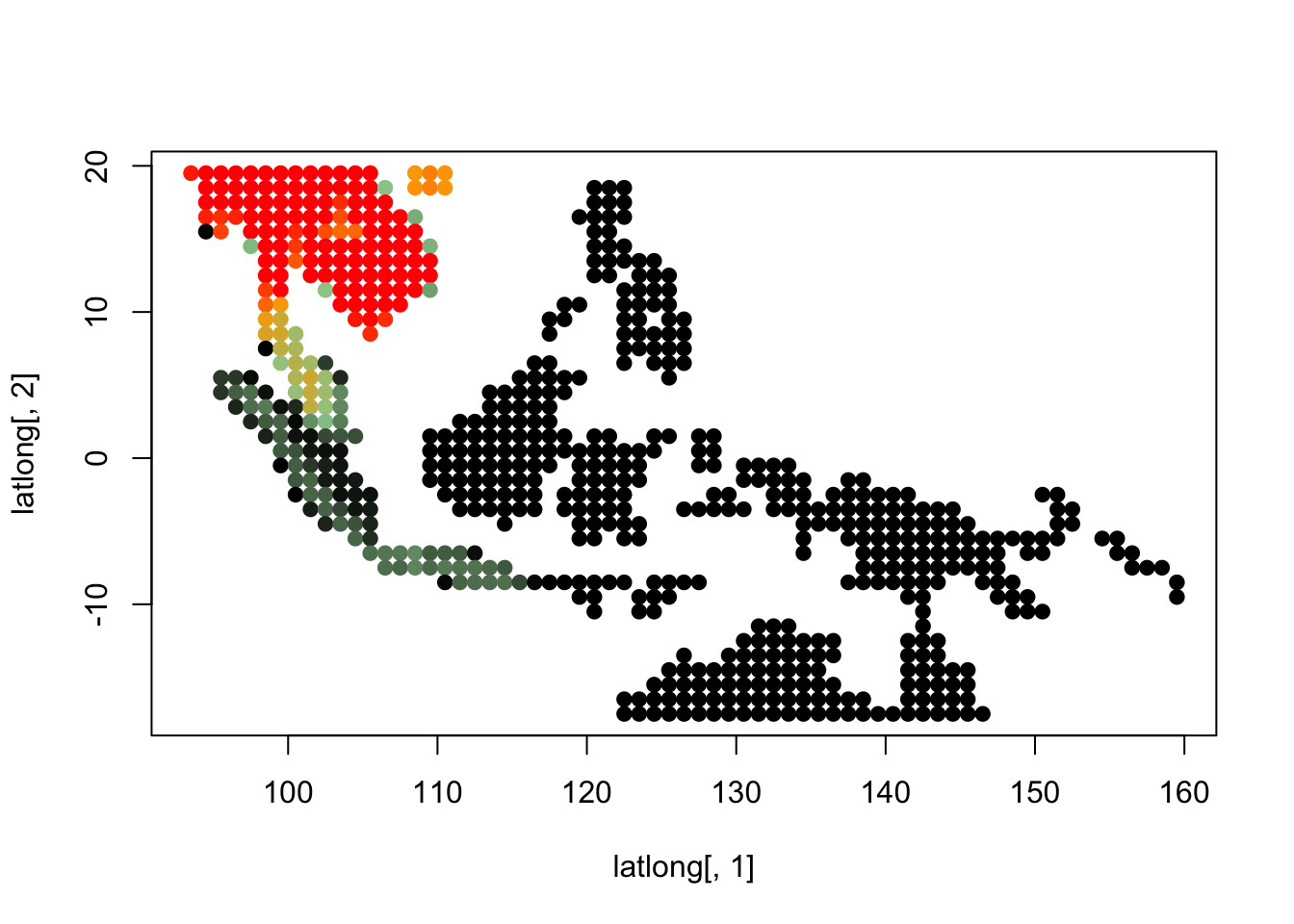
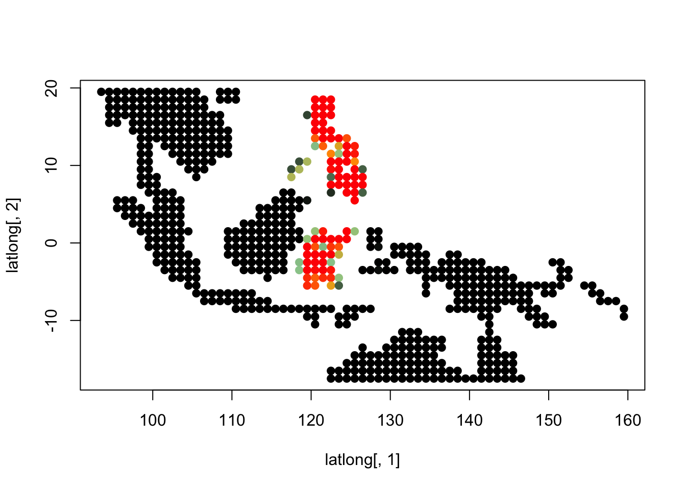
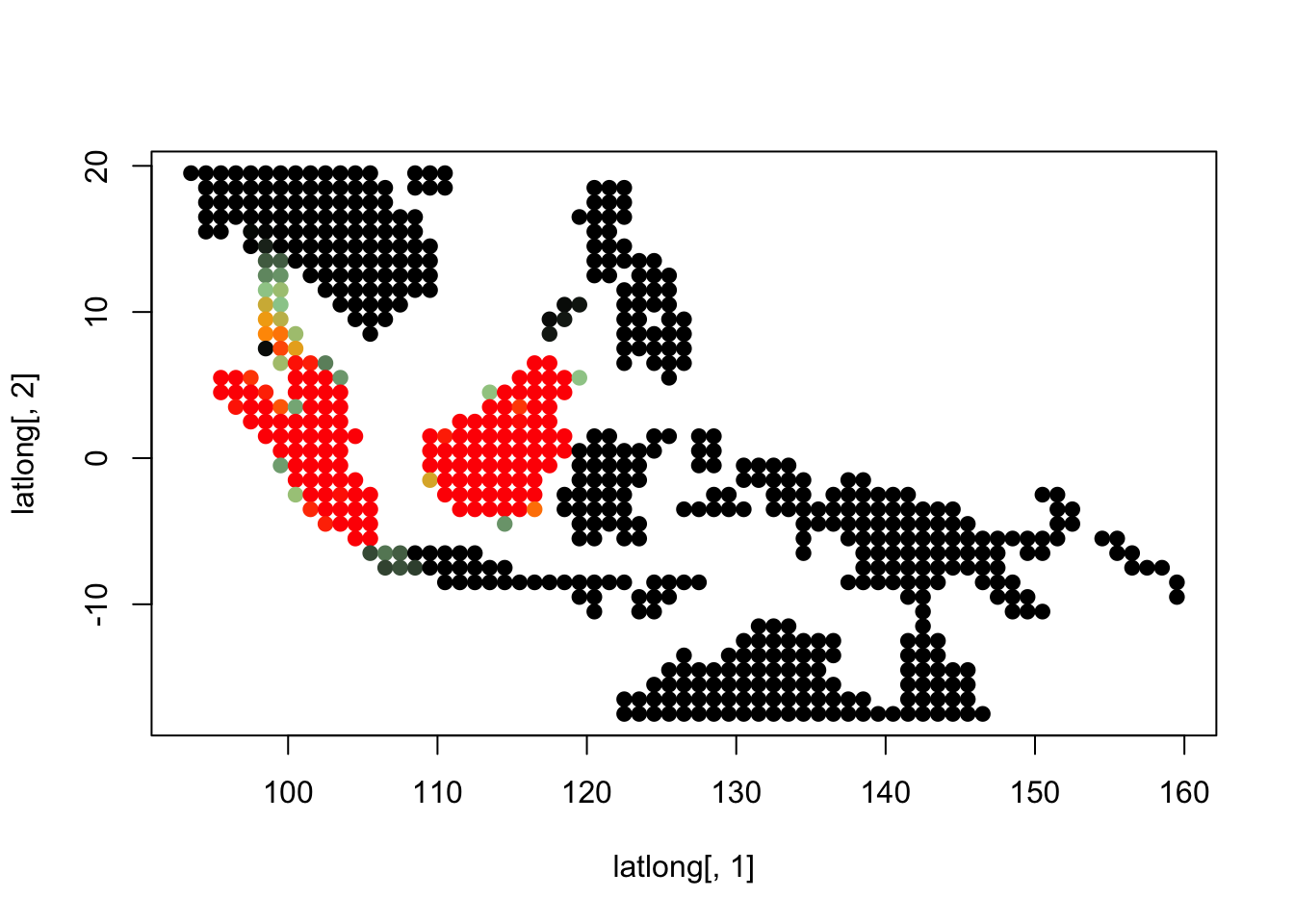
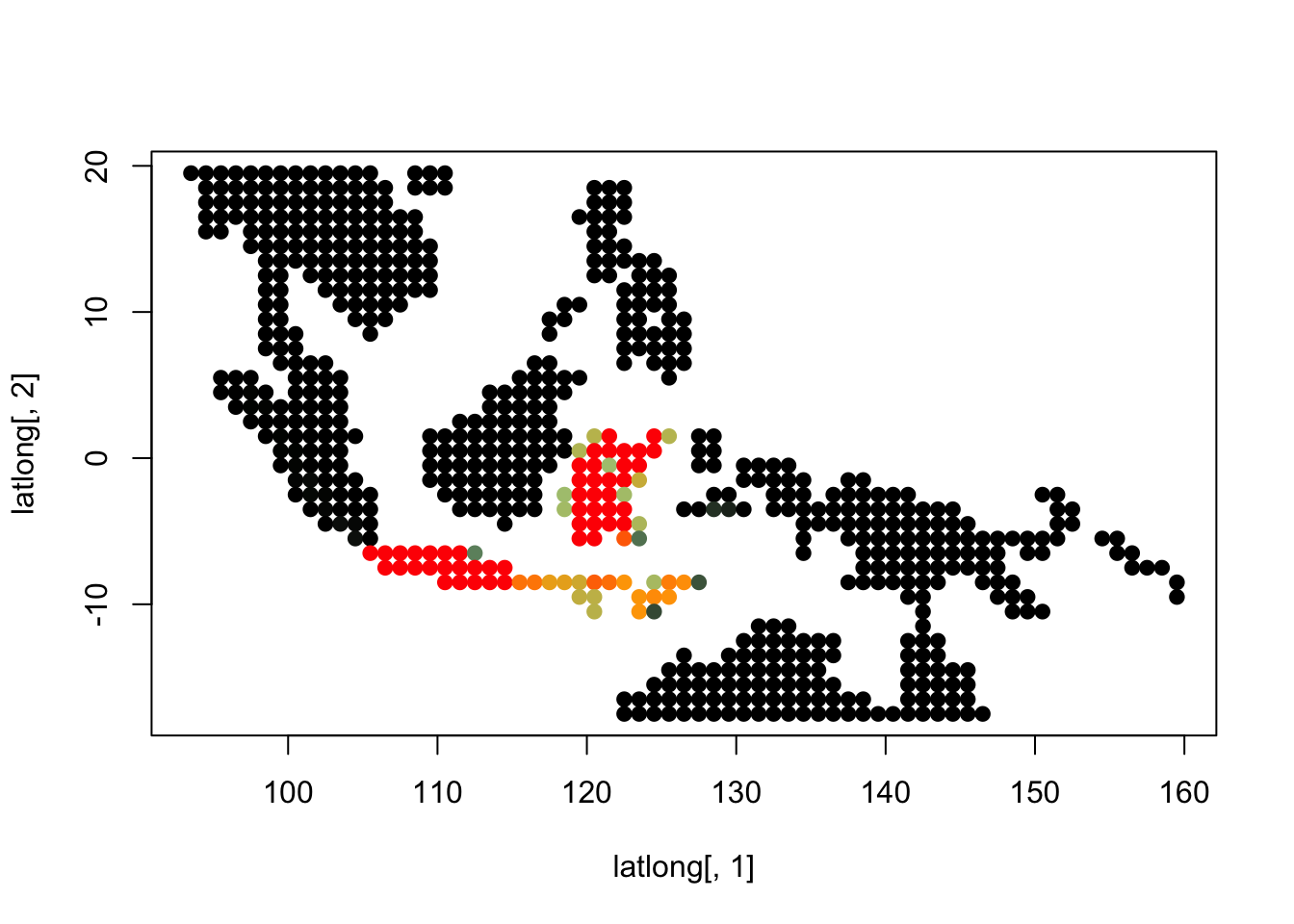
K = 5
topics <- topics_clust[[5]]
latlong_chars <- rownames(topics$freq)
latlong <- cbind.data.frame(as.numeric(sapply(latlong_chars,
              function(x) return(strsplit(x, "_")[[1]][1]))),
         as.numeric(sapply(latlong_chars,
              function(x) return(strsplit(x, "_")[[1]][2]))))

for(i in 1:dim(topics$freq)[2]){
  tmp <- round(1000*topics$freq[,i])+1
  colorGradient <- colorRampPalette(c("black", "darkseagreen3",
                                    "orange","red"))(1001)
  plot(latlong[,1], latlong[,2], col= colorGradient[tmp], pch = 20, cex = 1.5)
}
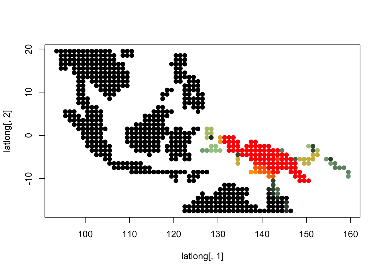
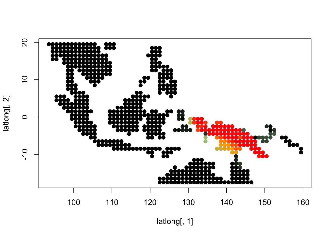
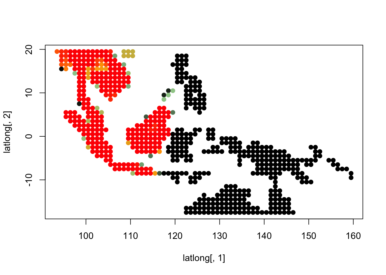
K = 7
topics <- topics_clust[[7]]
latlong_chars <- rownames(topics$freq)
latlong <- cbind.data.frame(as.numeric(sapply(latlong_chars,
              function(x) return(strsplit(x, "_")[[1]][1]))),
         as.numeric(sapply(latlong_chars,
              function(x) return(strsplit(x, "_")[[1]][2]))))

for(i in 1:dim(topics$freq)[2]){
  tmp <- round(1000*topics$freq[,i])+1
  colorGradient <- colorRampPalette(c("black", "darkseagreen3",
                                    "orange","red"))(1001)
  plot(latlong[,1], latlong[,2], col= colorGradient[tmp], pch = 20, cex = 1.5)
}

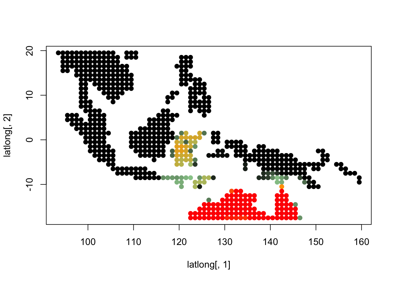
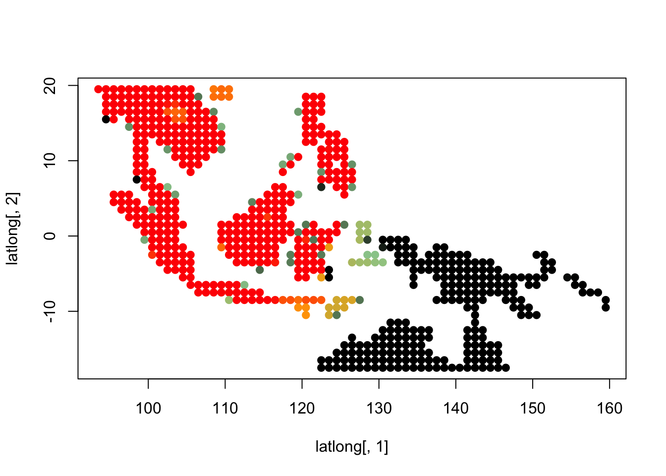
K = 10
topics <- topics_clust[[10]]
latlong_chars <- rownames(topics$freq)
latlong <- cbind.data.frame(as.numeric(sapply(latlong_chars,
              function(x) return(strsplit(x, "_")[[1]][1]))),
         as.numeric(sapply(latlong_chars,
              function(x) return(strsplit(x, "_")[[1]][2]))))

for(i in 1:dim(topics$freq)[2]){
  tmp <- round(1000*topics$freq[,i])+1
  colorGradient <- colorRampPalette(c("black", "darkseagreen3",
                                    "orange","red"))(1001)
  plot(latlong[,1], latlong[,2], col= colorGradient[tmp], pch = 20, cex = 1.5)
}


sessionInfo()## R version 3.5.0 (2018-04-23)
## Platform: x86_64-apple-darwin15.6.0 (64-bit)
## Running under: macOS Sierra 10.12.6
##
## Matrix products: default
## BLAS: /Library/Frameworks/R.framework/Versions/3.5/Resources/lib/libRblas.0.dylib
## LAPACK: /Library/Frameworks/R.framework/Versions/3.5/Resources/lib/libRlapack.dylib
##
## locale:
## [1] en_US.UTF-8/en_US.UTF-8/en_US.UTF-8/C/en_US.UTF-8/en_US.UTF-8
##
## attached base packages:
## [1] stats graphics grDevices utils datasets methods base
##
## other attached packages:
## [1] ggthemes_3.5.0 scales_0.5.0 mapplots_1.5
## [4] mapdata_2.3.0 maps_3.3.0 rgdal_1.2-20
## [7] gtools_3.5.0 rasterVis_0.44 latticeExtra_0.6-28
## [10] RColorBrewer_1.1-2 lattice_0.20-35 raster_2.6-7
## [13] sp_1.2-7 CountClust_1.6.1 ggplot2_2.2.1
## [16] methClust_0.1.0
##
## loaded via a namespace (and not attached):
## [1] zoo_1.8-1 modeltools_0.2-21 slam_0.1-43
## [4] reshape2_1.4.3 colorspace_1.3-2 htmltools_0.3.6
## [7] stats4_3.5.0 viridisLite_0.3.0 yaml_2.1.19
## [10] mgcv_1.8-23 rlang_0.2.0 hexbin_1.27.2
## [13] pillar_1.2.2 plyr_1.8.4 stringr_1.3.1
## [16] munsell_0.4.3 gtable_0.2.0 evaluate_0.10.1
## [19] labeling_0.3 knitr_1.20 permute_0.9-4
## [22] flexmix_2.3-14 parallel_3.5.0 Rcpp_0.12.17
## [25] backports_1.1.2 limma_3.36.1 vegan_2.5-1
## [28] maptpx_1.9-5 picante_1.7 digest_0.6.15
## [31] stringi_1.2.2 cowplot_0.9.2 grid_3.5.0
## [34] rprojroot_1.3-2 tools_3.5.0 magrittr_1.5
## [37] lazyeval_0.2.1 tibble_1.4.2 cluster_2.0.7-1
## [40] ape_5.1 MASS_7.3-49 Matrix_1.2-14
## [43] SQUAREM_2017.10-1 assertthat_0.2.0 rmarkdown_1.9
## [46] boot_1.3-20 nnet_7.3-12 nlme_3.1-137
## [49] compiler_3.5.0This R Markdown site was created with workflowr