Phylogenetic analysis of Wallacea bird species - no seabirds

Intro

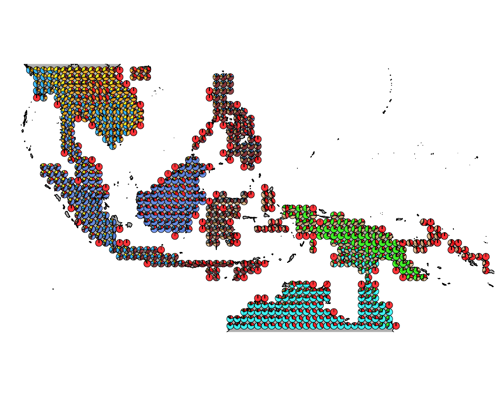
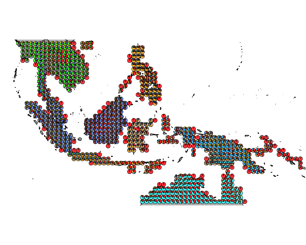
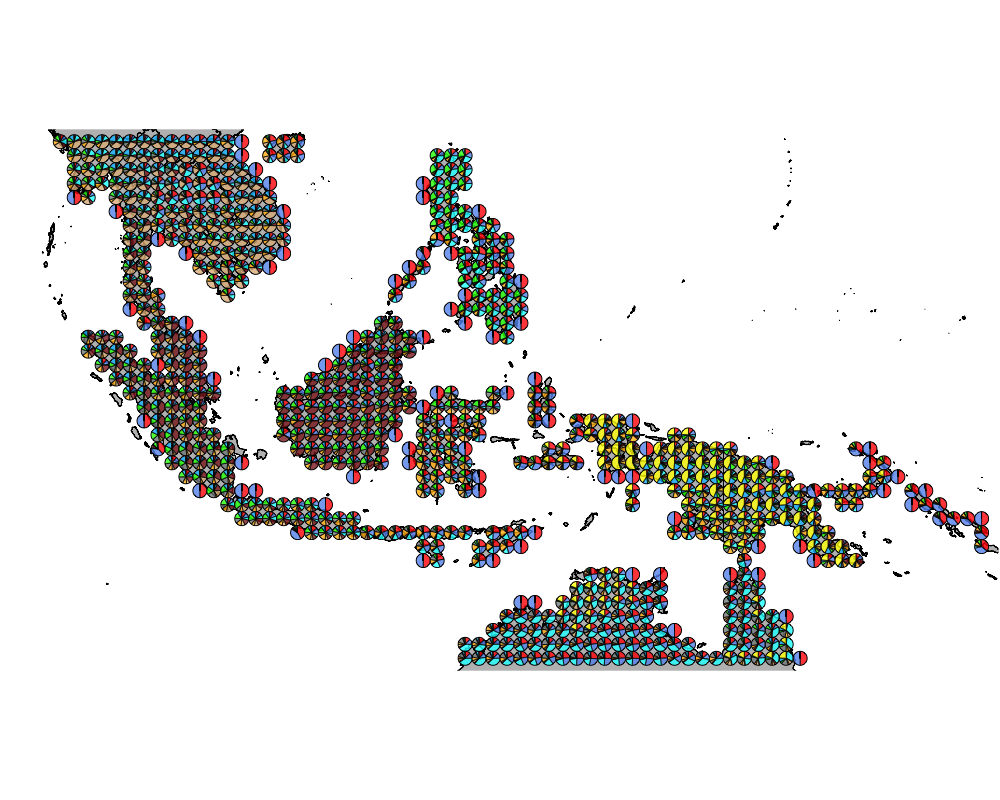
We use the phylogenetic information on bird species to combine them at different stages of history going up from current time, that corresponds to all the reported species. Then GoM model was run on the combined species at each cut off of the phylogentic tree and the resultant grouping. Here we concentrate on the bird species from Wallacea except the sea birds.

Packages

library(methClust)
library(CountClust)
library(rasterVis)
library(gtools)
library(sp)
library(rgdal)
library(ggplot2)
library(maps)
library(mapdata)
library(mapplots)
library(scales)
library(ggthemes)
library(ape)
library(phytools)

Data

We look at phylogenetic analyses of the bird species in Wallacea.

library(ape)
MyTree <- read.tree("../data/wallaces_line_trees_mean_no_seabirds.nwk")

datalist <- get(load("../data/wallace_region_pres_ab_breeding_no_seabirds.rda"))
latlong <- datalist$loc
data <- datalist$dat

Data + phylogeny

names_phylogeny_match <- read.csv("../data/names_matched_to_phylogeny.csv", 
                                  header = TRUE, row.names = 1)

tip_labels <- MyTree$tip.label
tip_labels <- gsub("_", " ", tip_labels)
common_names <- intersect(colnames(data), names_phylogeny_match[,1])
data2 <- data[, match(common_names, colnames(data))]

new_names <- names_phylogeny_match[match(colnames(data2), names_phylogeny_match[,1]),2]
colnames(data2) <- new_names

idx2 <- match(tip_labels, as.character(names_phylogeny_match[,2]))

newTree <- MyTree
newTree$tip.label <- tip_labels

source("../code/collapse_counts_by_phylo.R")
sliced_data_cutoffs <- list()
k <- 1
for(cut in c(5, 10, 15, 20, 30, 40, 50, 60, 70, 75, 80)){
  sliced_data_cutoffs[[k]] <- collapse_counts_by_phylo(data2, newTree, collapse_at = cut)
  k  =  k + 1
}
save(sliced_data_cutoffs, file = "../output/sliced_data_cutoffs.rda")

GoM model

Here we show a demo of the code of applying ecoStructure with K=2 at different cut offs of the counts data.

topic_clust <- list()
for(k in 1:length(cuts)){
  num_groups_mat <- t(sliced_data_cutoffs[[k]]$num_groups %*% t(rep(1, dim(data2)[1])))
  meth <- sliced_data_cutoffs[[k]]$outdat
  unmeth <- num_groups_mat - meth
  topic_clust[[k]] <- meth_topics(meth, unmeth, K=2, tol = 0.1, use_squarem = FALSE)
}

save(topic_clust, file = "../output/phylogenetic_wallacea_methClust_2.rda")

Visualization

for(id in 2:10){
  topic_clust <- get(load(paste0("../output/phylo_meth/phylogenetic_wallacea_methClust_", id, ".rda")))

color = c("red", "cornflowerblue", "cyan", "brown4", "burlywood", "darkgoldenrod1",
          "azure4", "green","deepskyblue","yellow", "azure1")
intensity <- 0.8
for(k in 1:length(cuts)){
    png(filename=paste0("../docs/phylogenetic_wallacea/clus_", id, "/cutoff_", cuts[k], ".png"),width = 1000, height = 800)
  map("worldHires",
      ylim=c(-18,20), xlim=c(90,160), # Re-defines the latitude and longitude range
      col = "gray", fill=TRUE, mar=c(0.1,0.1,0.1,0.1))
  lapply(1:dim(topic_clust[[k]]$omega)[1], function(r)
    add.pie(z=as.integer(100*topic_clust[[k]]$omega[r,]),
            x=latlong[r,1], y=latlong[r,2], labels=c("","",""),
            radius = 0.5,
            col=c(alpha(color[1],intensity),alpha(color[2],intensity),
                  alpha(color[3], intensity), alpha(color[4], intensity),
                  alpha(color[5], intensity), alpha(color[6], intensity),
                  alpha(color[7], intensity), alpha(color[8], intensity),
                  alpha(color[9], intensity), alpha(color[10], intensity),
                  alpha(color[11], intensity))));
  dev.off()
  }
}

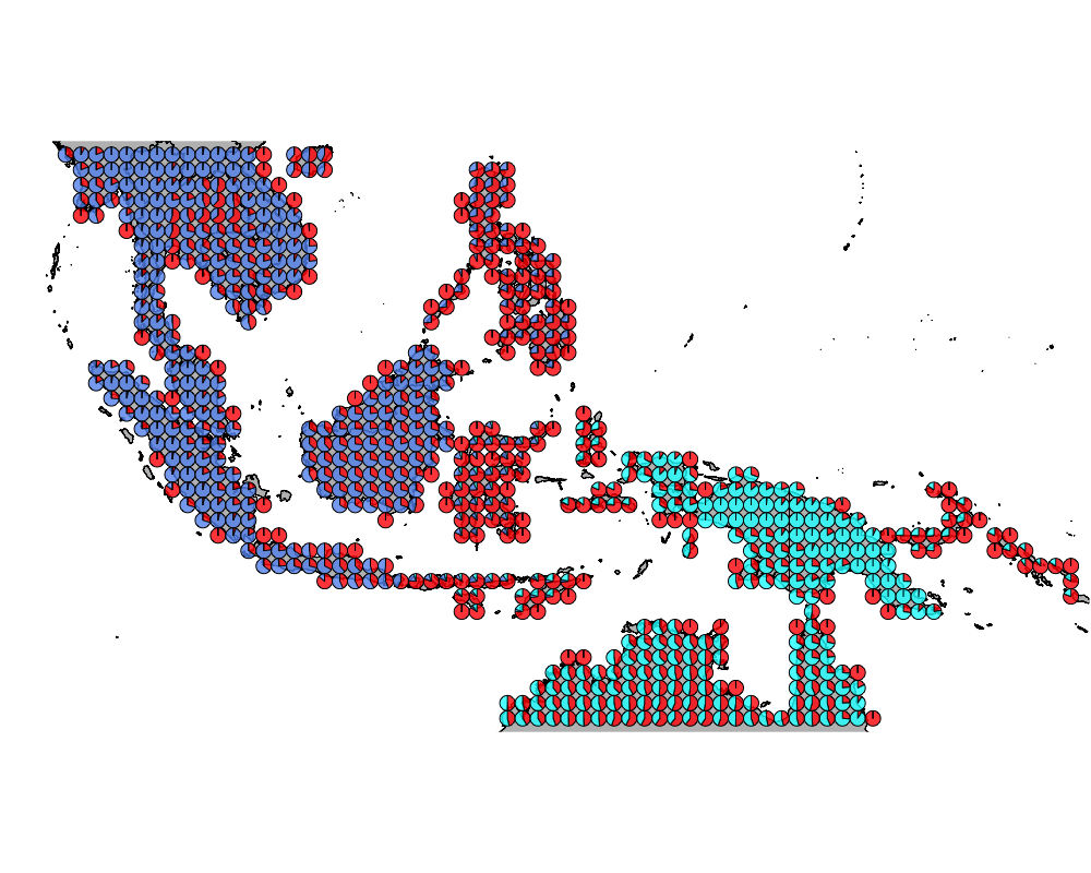
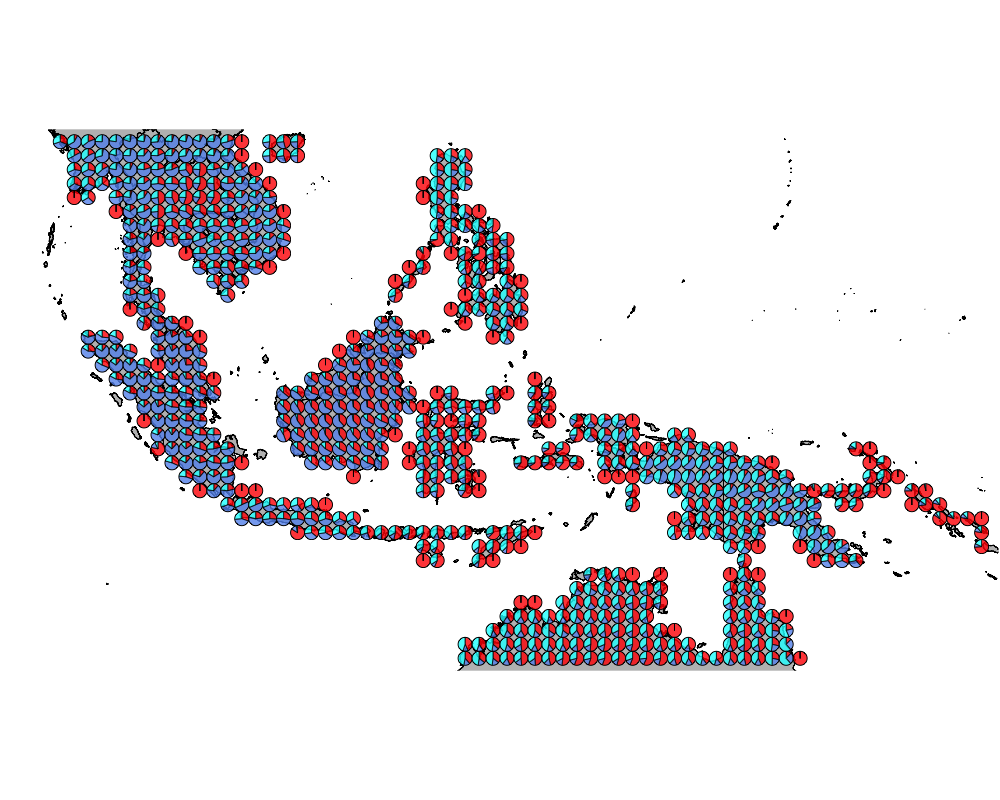
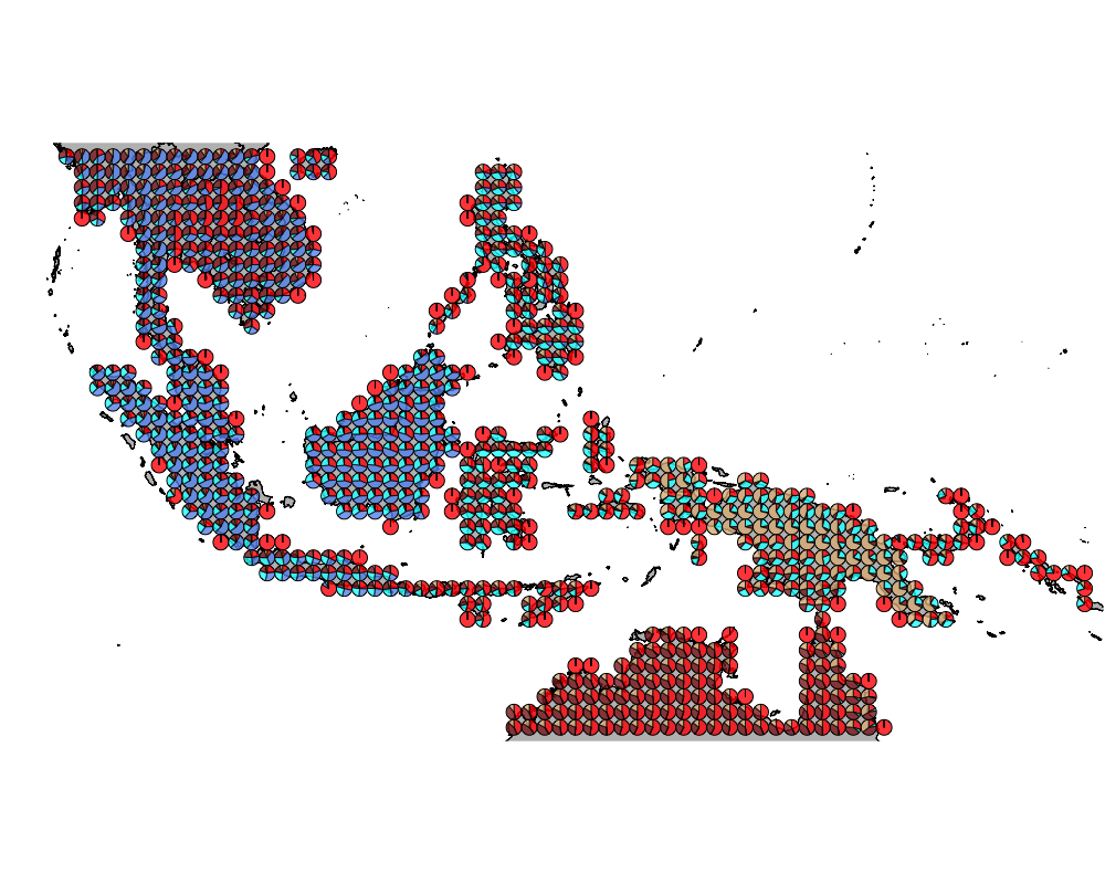
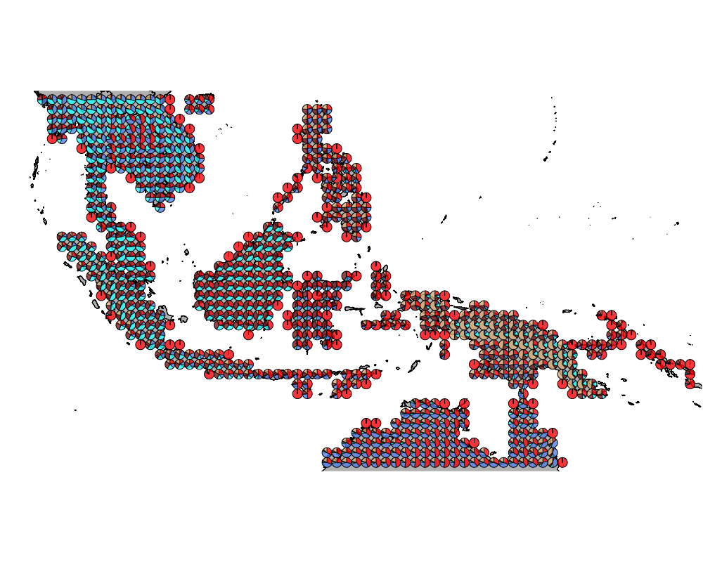
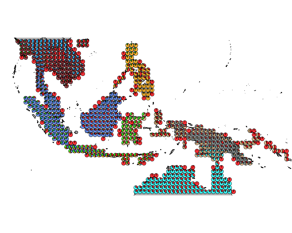
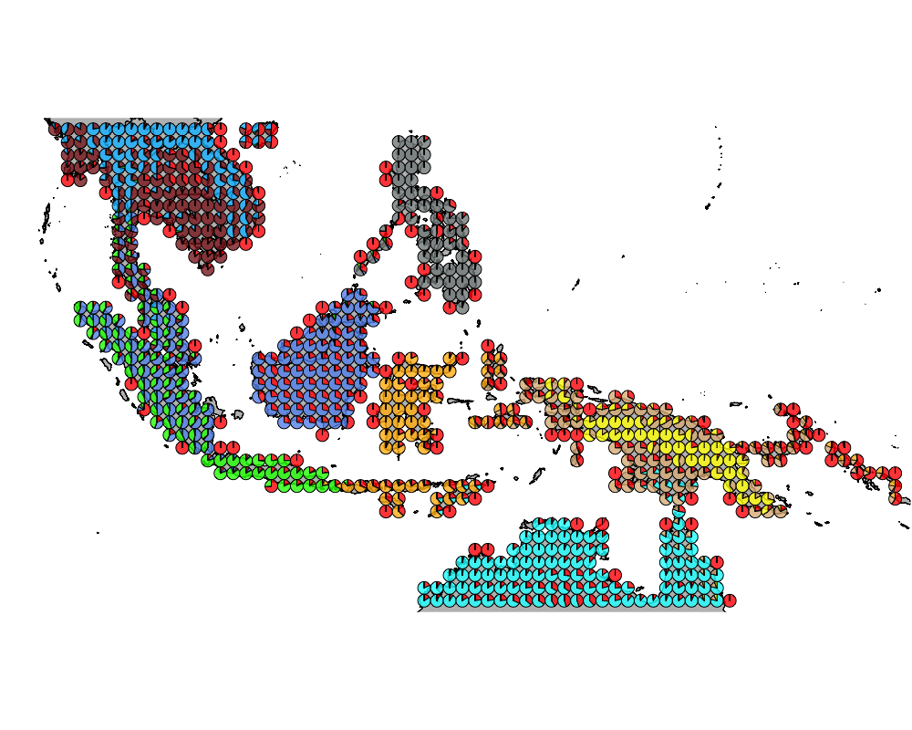
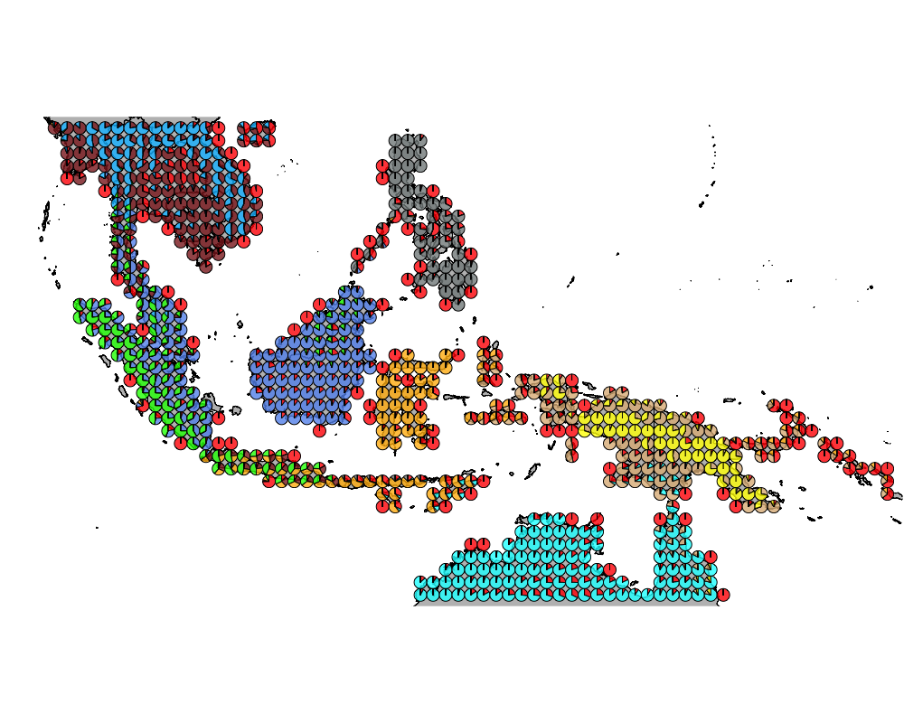
K = 2

cut-off = 5

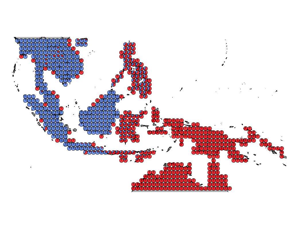
cutoff1

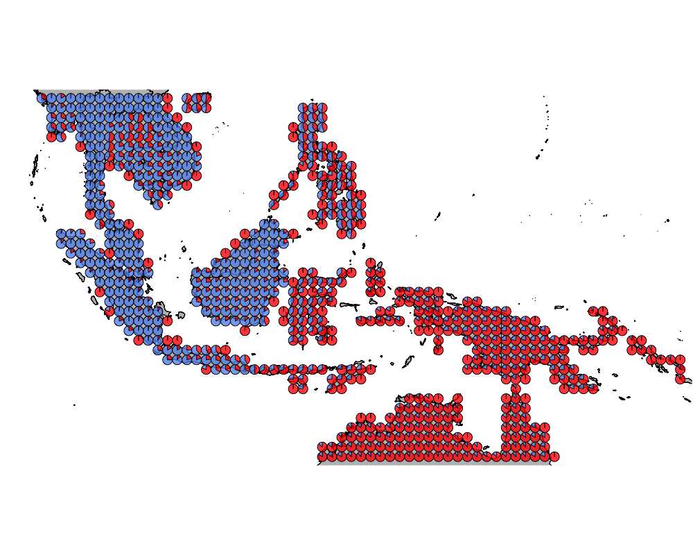
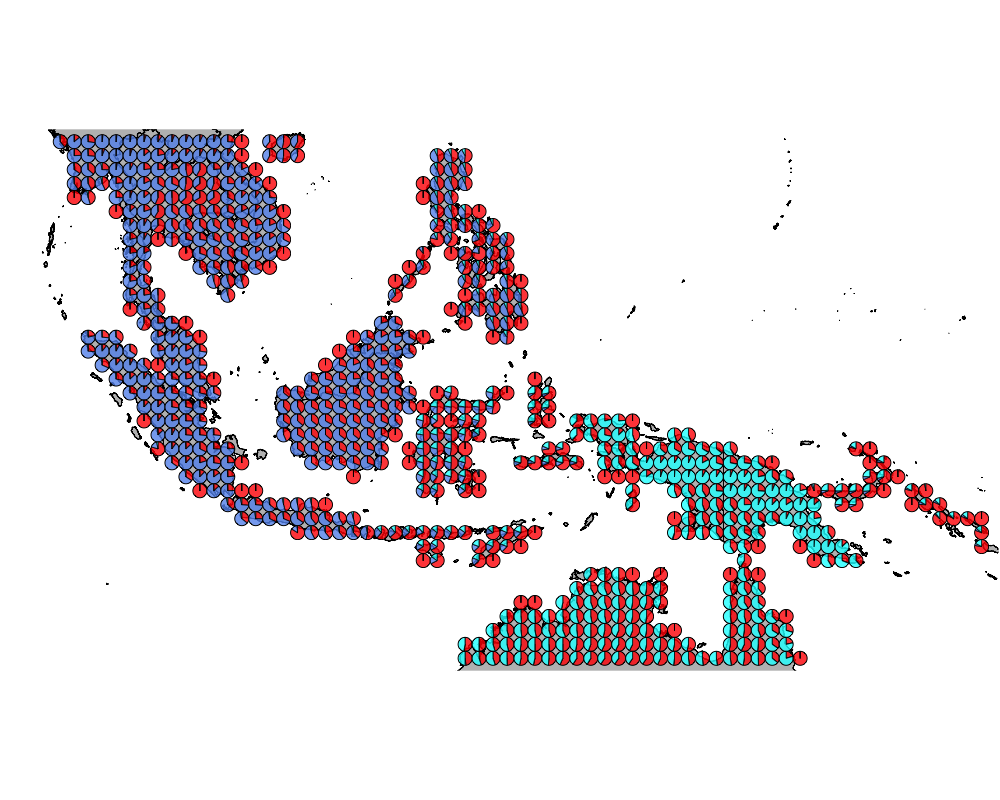
cut-off = 10

cutoff2

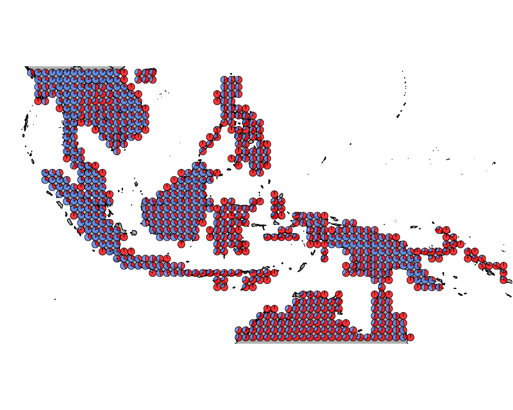
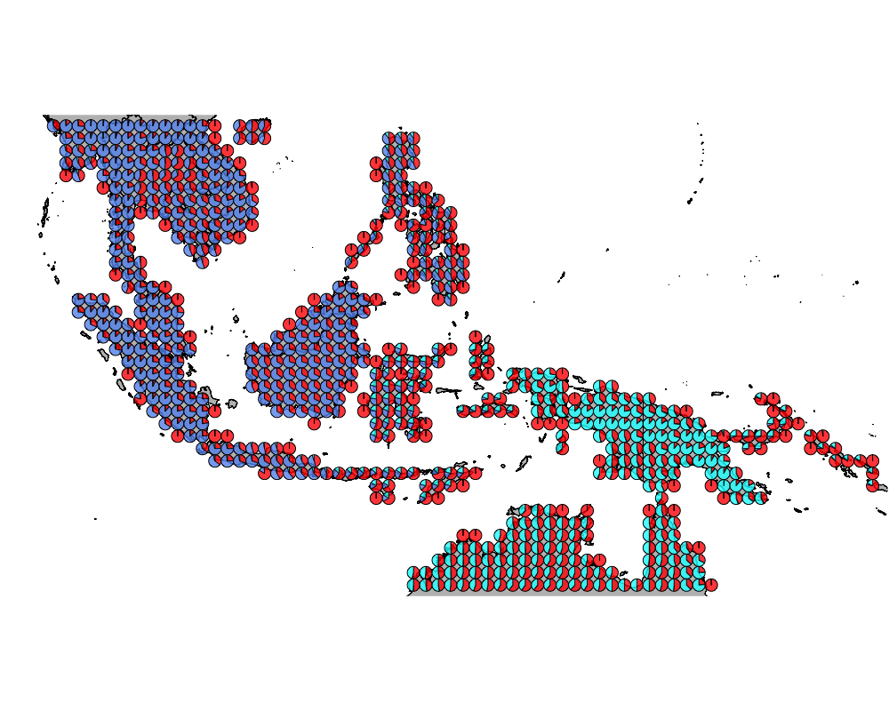
cut-off = 30

cutoff5

cut-off = 40

cutoff6

cut-off = 50

cutoff7

cut-off = 60

cutoff8

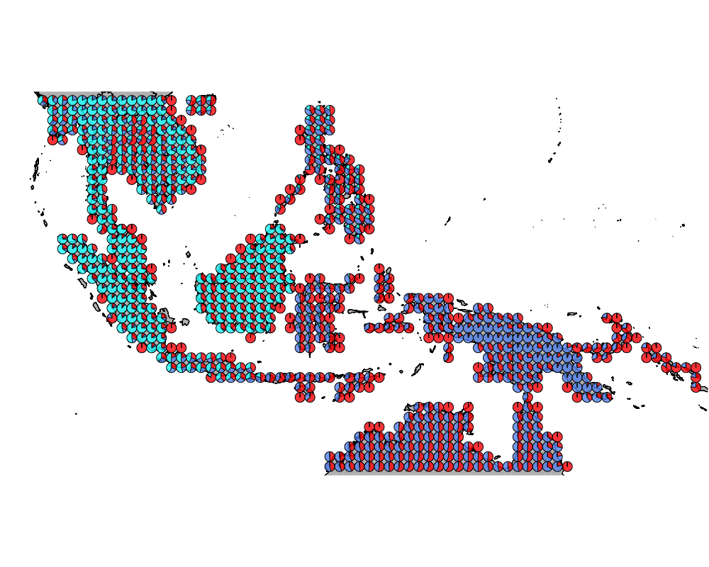
cut-off = 80

cutoff11

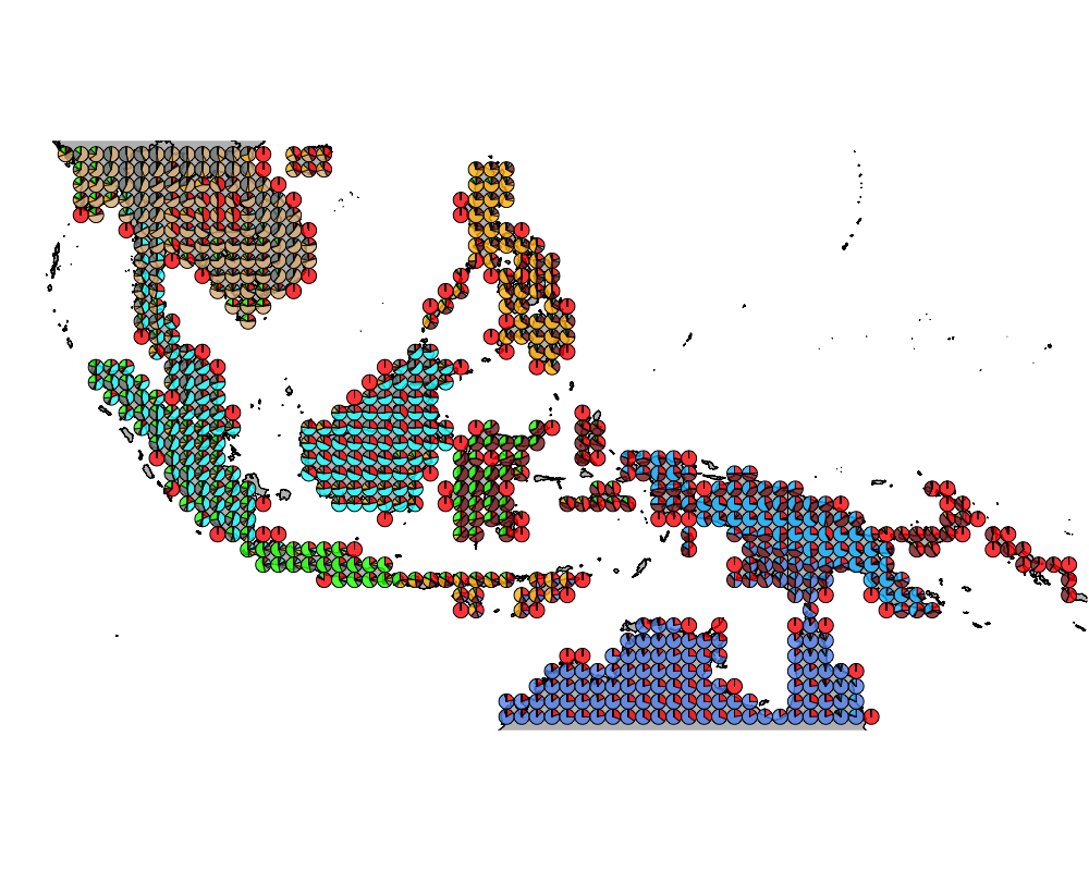
K = 3

cut-off = 5

cutoff1

cut-off = 10

cutoff1

cut-off = 30

cutoff1

cut-off = 40

cutoff1

cut-off = 50

cutoff1

cut-off = 60

cutoff1

cut-off = 80

cutoff1

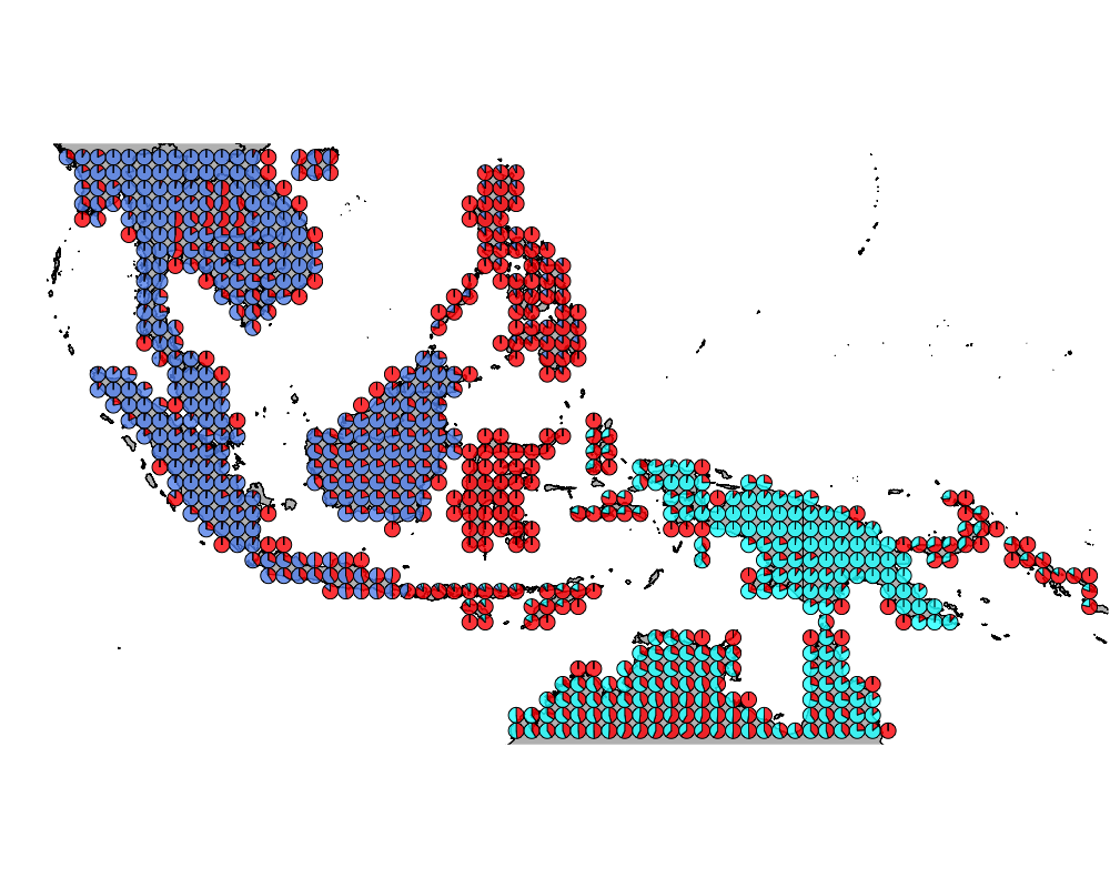
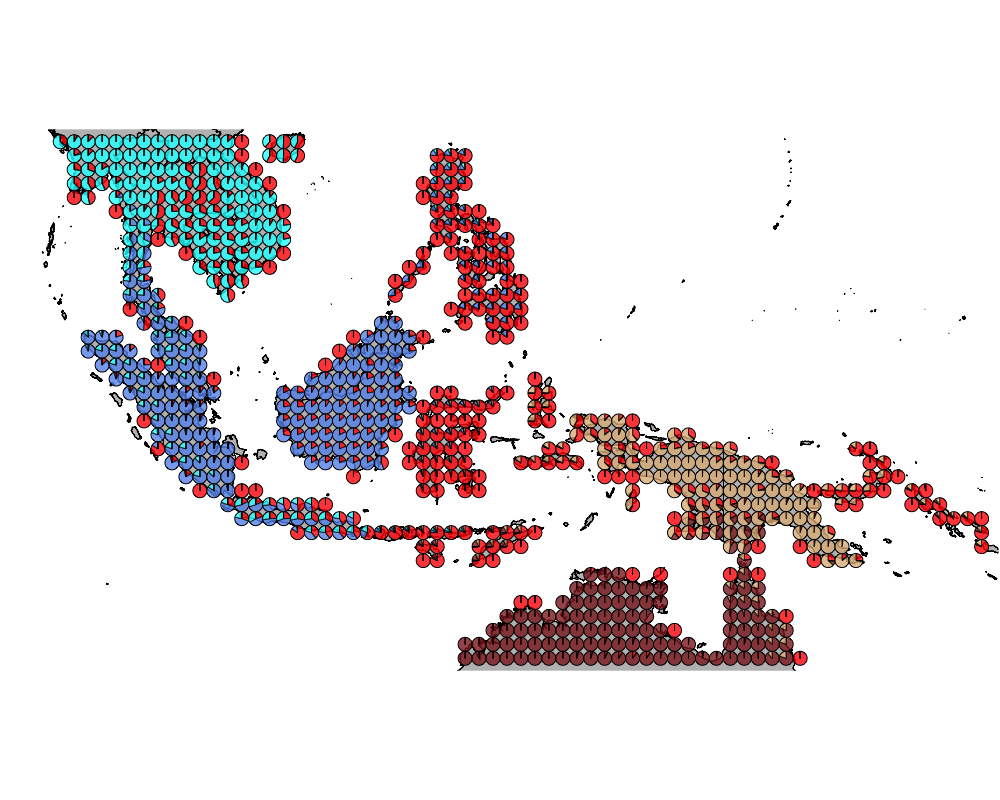
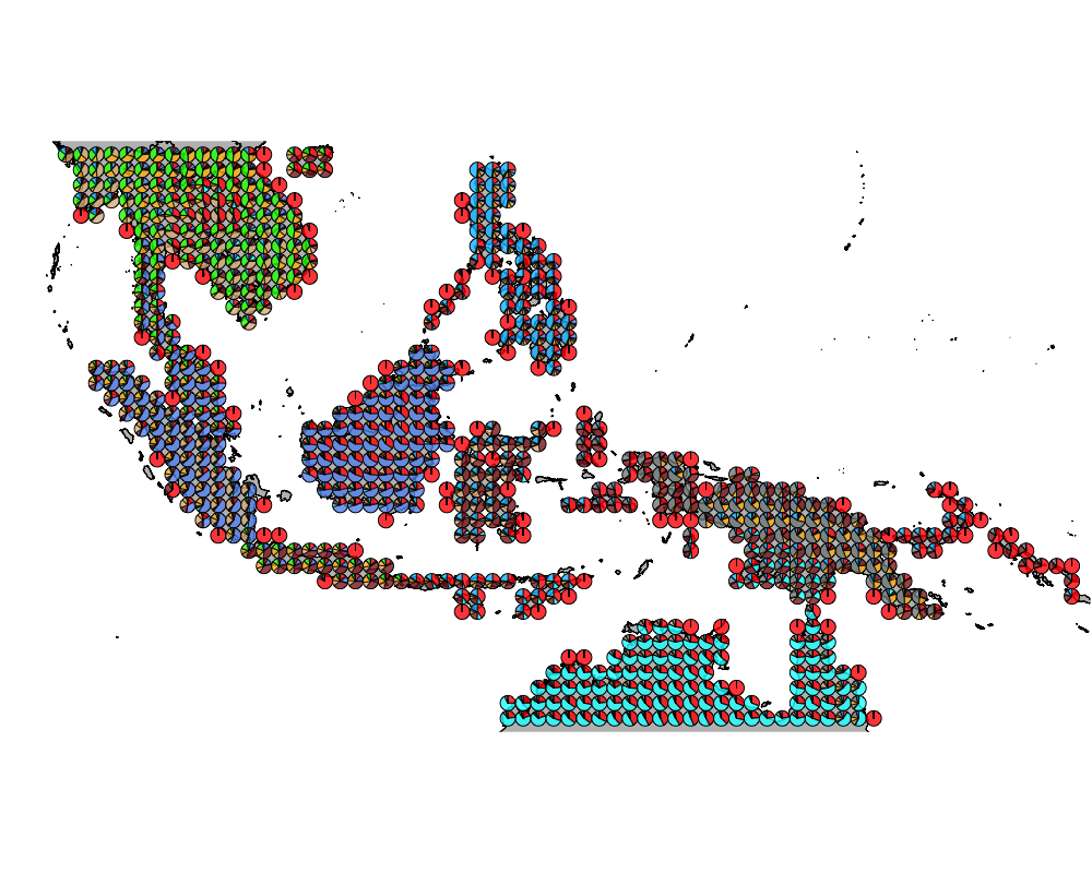
K = 5

cut-off = 5

cutoff1

cut-off = 10

cutoff1

cut-off = 30

cutoff1

cut-off = 40

cutoff1

cut-off = 50

cutoff1

cut-off = 60

cutoff1

cut-off = 80

cutoff1

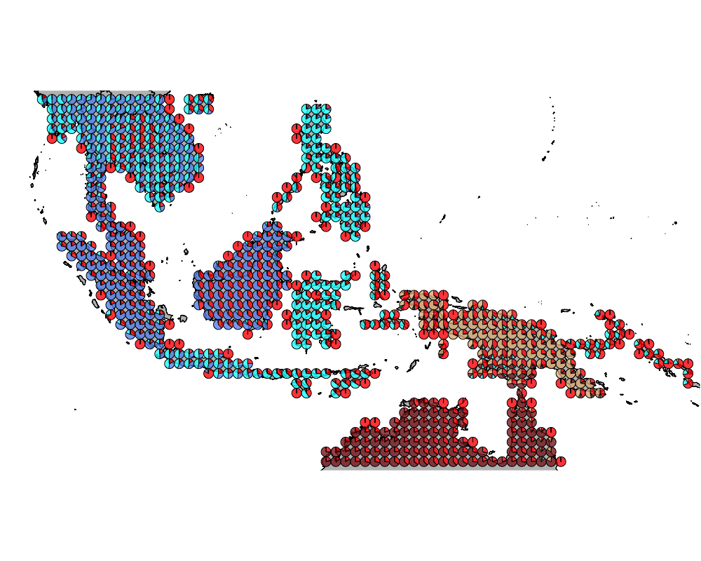
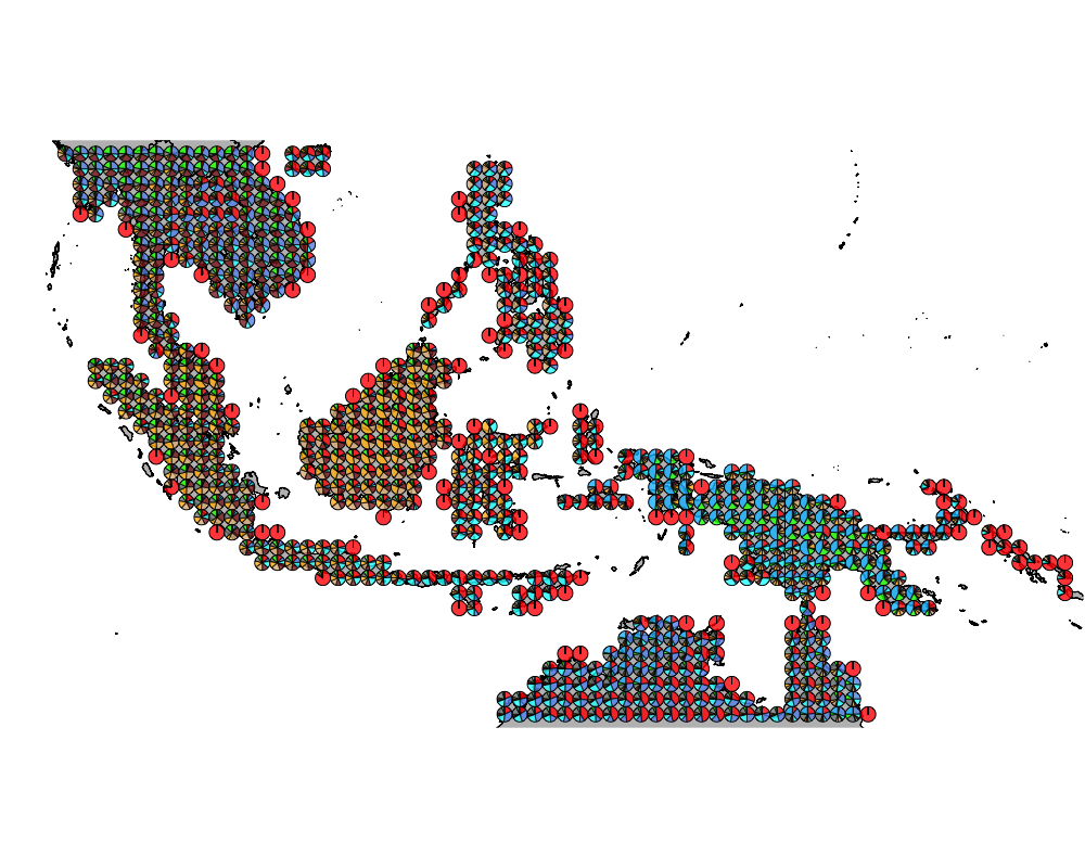
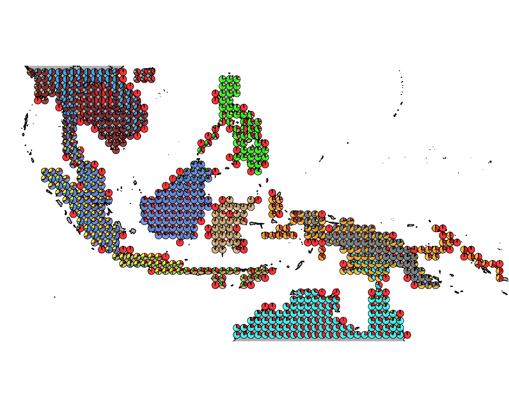
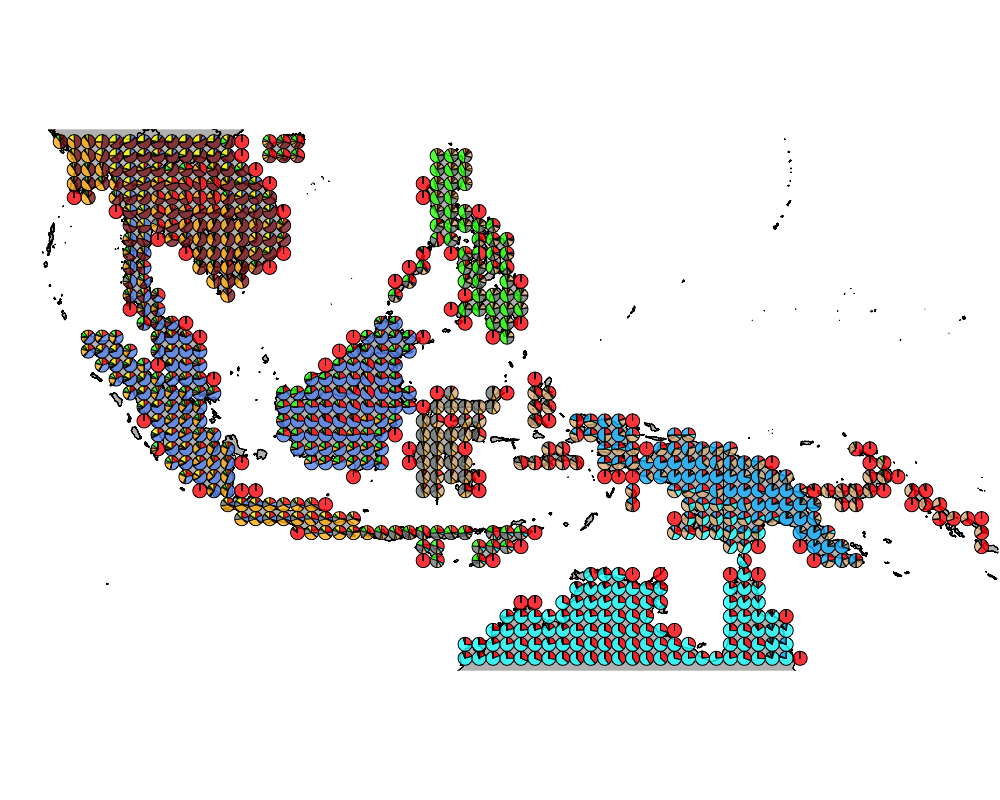
K = 9

cut-off = 5

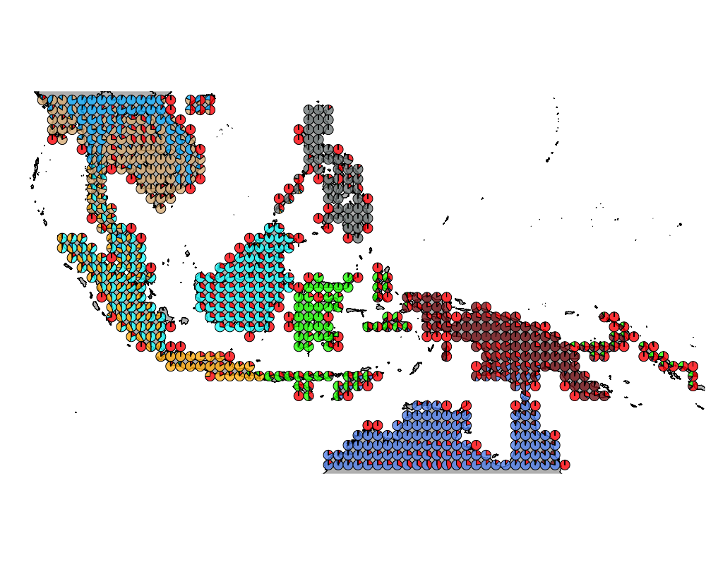
cutoff1

cut-off = 10

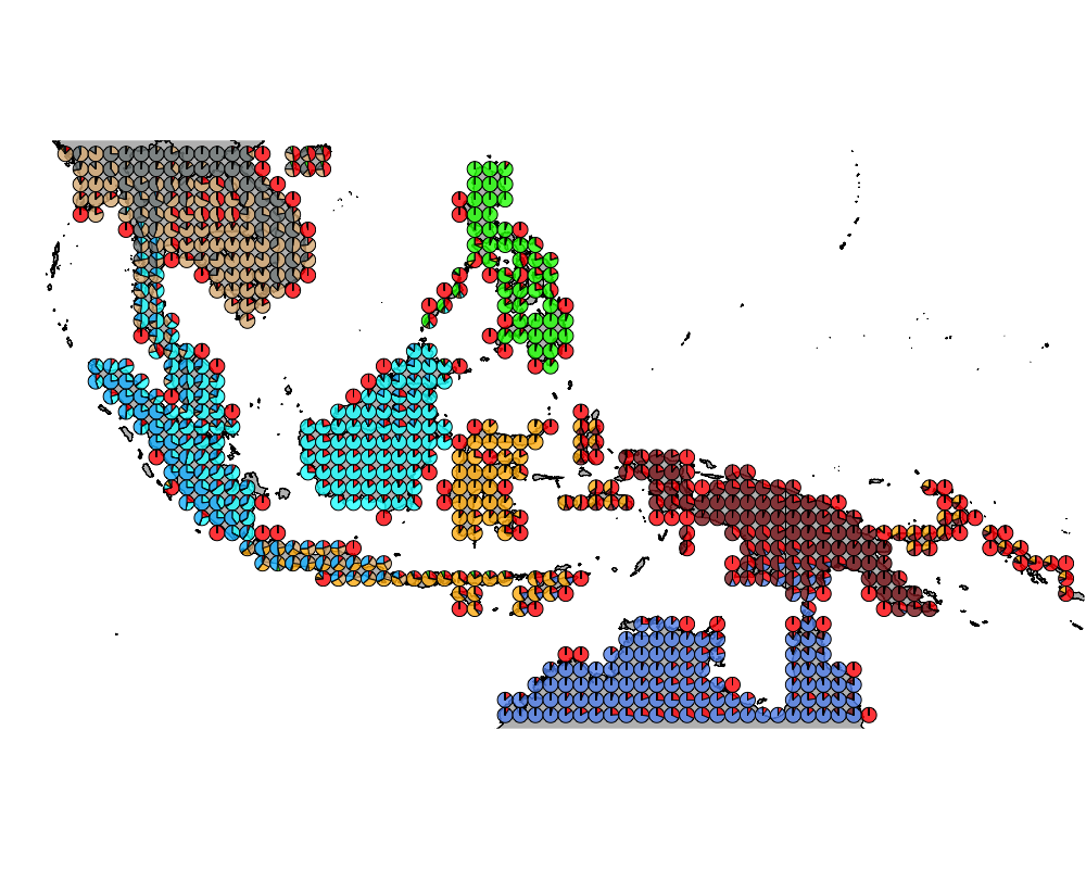
cutoff1

cut-off = 30

cutoff1

cut-off = 40

cutoff1

cut-off = 50

cutoff1

cut-off = 60

cutoff1

cut-off = 80

cutoff1

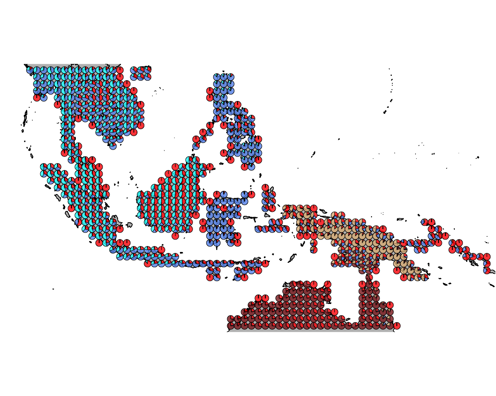
K = 10

cut-off = 5

cutoff1

cut-off = 10

cutoff1

cut-off = 30

cutoff1

cut-off = 40

cutoff1

cut-off = 50

cutoff1

cut-off = 60

cutoff1

cut-off = 80

cutoff1

SessionInfo

sessionInfo()

## R version 3.4.4 (2018-03-15)
## Platform: x86_64-apple-darwin15.6.0 (64-bit)
## Running under: macOS Sierra 10.12.6
## 
## Matrix products: default
## BLAS: /Library/Frameworks/R.framework/Versions/3.4/Resources/lib/libRblas.0.dylib
## LAPACK: /Library/Frameworks/R.framework/Versions/3.4/Resources/lib/libRlapack.dylib
## 
## locale:
## [1] en_US.UTF-8/en_US.UTF-8/en_US.UTF-8/C/en_US.UTF-8/en_US.UTF-8
## 
## attached base packages:
## [1] stats     graphics  grDevices utils     datasets  methods   base     
## 
## other attached packages:
##  [1] phytools_0.6-44     ape_5.0             ggthemes_3.4.0     
##  [4] scales_0.5.0.9000   mapplots_1.5        mapdata_2.2-6      
##  [7] maps_3.2.0          rgdal_1.2-16        gtools_3.5.0       
## [10] rasterVis_0.41      latticeExtra_0.6-28 RColorBrewer_1.1-2 
## [13] lattice_0.20-35     raster_2.6-7        sp_1.2-7           
## [16] CountClust_1.5.1    ggplot2_2.2.1       methClust_0.1.0    
## 
## loaded via a namespace (and not attached):
##  [1] viridisLite_0.3.0       splines_3.4.4          
##  [3] assertthat_0.2.0        expm_0.999-2           
##  [5] stats4_3.4.4            animation_2.5          
##  [7] yaml_2.1.18             slam_0.1-42            
##  [9] numDeriv_2016.8-1       pillar_1.1.0           
## [11] backports_1.1.2         quadprog_1.5-5         
## [13] limma_3.34.9            phangorn_2.3.1         
## [15] digest_0.6.15           colorspace_1.3-2       
## [17] picante_1.6-2           cowplot_0.9.2          
## [19] htmltools_0.3.6         Matrix_1.2-12          
## [21] plyr_1.8.4              pkgconfig_2.0.1        
## [23] mvtnorm_1.0-6           combinat_0.0-8         
## [25] tibble_1.4.2            mgcv_1.8-23            
## [27] nnet_7.3-12             hexbin_1.27.1          
## [29] lazyeval_0.2.1          mnormt_1.5-5           
## [31] survival_2.41-3         magrittr_1.5           
## [33] evaluate_0.10.1         msm_1.6.5              
## [35] nlme_3.1-131.1          MASS_7.3-47            
## [37] vegan_2.4-4             tools_3.4.4            
## [39] stringr_1.3.0           munsell_0.4.3          
## [41] plotrix_3.7             cluster_2.0.6          
## [43] compiler_3.4.4          clusterGeneration_1.3.4
## [45] rlang_0.2.0             grid_3.4.4             
## [47] igraph_1.1.2            rmarkdown_1.9          
## [49] boot_1.3-20             gtable_0.2.0           
## [51] flexmix_2.3-14          reshape2_1.4.3         
## [53] zoo_1.8-0               knitr_1.20             
## [55] fastmatch_1.1-0         rprojroot_1.3-2        
## [57] maptpx_1.9-3            permute_0.9-4          
## [59] modeltools_0.2-21       stringi_1.1.6          
## [61] parallel_3.4.4          SQUAREM_2017.10-1      
## [63] Rcpp_0.12.16            coda_0.19-1            
## [65] scatterplot3d_0.3-40