Phylogenetic analysis of Indonesian bird species
Kushal K Dey
4/2/2018
Intro
We use the phylogenetic information on bird species to combine them at different stages of history going up from current time, that corresponds to all the reported species. Then GoM model was run on the combined species at each cut off of the phylogentic tree and the resultant grouping. Here we concentrate on only the bird species from Java, Bali, Lombok and Sumbawa.
Packages
library(methClust)
library(CountClust)
library(rasterVis)
library(gtools)
library(sp)
library(rgdal)
library(ggplot2)
library(maps)
library(mapdata)
library(mapplots)
library(scales)
library(ggthemes)
library(ape)
library(phytools)
Data
library(ape)
MyTree <- read.tree("../data/wallaces_line_trees_mean_no_seabirds.nwk")
datalist <- get(load("../data/wallace_region_pres_ab_breeding_no_seabirds.rda"))
latlong <- datalist$loc
data <- datalist$dat
idx1 <- which(latlong[,2] > -9.3 & latlong[,2] < -7.3)
idx2 <- which(latlong[,1] > 112 & latlong[,1] < 119.5)
idx <- intersect(idx1, idx2)
length(idx)## [1] 10latlong2 <- latlong[idx,]
birds_pa_data_2 <- data[idx, ]
birds_pa_data_3 <- birds_pa_data_2[, which(colSums(birds_pa_data_2)!=0)]Processing data + phylogeny
data <- birds_pa_data_3
names_phylogeny_match <- read.csv("../data/names_matched_to_phylogeny.csv",
                                  header = TRUE, row.names = 1)

tip_labels <- MyTree$tip.label
tip_labels <- gsub("_", " ", tip_labels)
common_names <- intersect(colnames(data), names_phylogeny_match[,1])
data2 <- data[, match(common_names, colnames(data))]

new_names <- names_phylogeny_match[match(colnames(data2), names_phylogeny_match[,1]),2]
colnames(data2) <- new_names

idx2 <- match(tip_labels, as.character(names_phylogeny_match[,2]))

newTree <- MyTree
newTree$tip.label <- tip_labels
source("../code/collapse_counts_by_phylo.R")
sliced_data_cutoffs <- list()
k <- 1
for(cut in c(5, 10, 15, 20, 30, 40, 50, 60, 70, 75, 80, 85, 90, 95, 100)){
sliced_data_cutoffs[[k]] <- collapse_counts_by_phylo(data2, newTree, collapse_at = cut)
k = k + 1
}
save(sliced_data_cutoffs, file = "../output/sliced_data_cutoffs_indonesia.rda")GoM model
cuts <- c(5, 10, 15, 20, 30, 40, 50, 60, 70, 75, 80, 85, 90, 95, 100)
topic_clust <- list()
for(k in 1:length(cuts)){
  num_groups_mat <- t(sliced_data_cutoffs[[k]]$num_groups %*% t(rep(1, dim(data2)[1])))
  meth <- sliced_data_cutoffs[[k]]$outdat
  unmeth <- num_groups_mat - meth
  topic_clust[[k]] <- meth_topics(meth, unmeth, K=2, tol = 0.01, use_squarem = FALSE)
}
##
## Estimating on a 10 samples collection.
## log posterior increase: 967.46, 0.03, -1.12, 0.97, 0.31, 0.23, 0, done.
##
## Estimating on a 10 samples collection.
## log posterior increase: 7531.88, 49.42, 0.09, 0.01, 3.73, 0.44, 0.32, 0.27, 0.83, done.
##
## Estimating on a 10 samples collection.
## log posterior increase: 593.56, 0, 2.27, done.
##
## Estimating on a 10 samples collection.
## log posterior increase: 1270.56, 0.09, done.
##
## Estimating on a 10 samples collection.
## log posterior increase: 1110.56, 0.09, 0.03, 1.47, 0, done.
##
## Estimating on a 10 samples collection.
## log posterior increase: 171.46, 0.01, done.
##
## Estimating on a 10 samples collection.
## log posterior increase: 102.68, 0.04, 0, done.
##
## Estimating on a 10 samples collection.
## log posterior increase: 110.23, 0.02, done.
##
## Estimating on a 10 samples collection.
## log posterior increase: 203.98, 0.3, 0.73, 0.01, done.
##
## Estimating on a 10 samples collection.
## log posterior increase: 154.65, 0.48, 0.13, 0.07, 0.04, 0.03, 0.02, 0.02, 0.01, 0.01, done.
##
## Estimating on a 10 samples collection.
## log posterior increase: 103.06, 0.55, 0.15, 0.07, 0.05, 0.03, 0.02, 0.02, 0.01, done.
##
## Estimating on a 10 samples collection.
## log posterior increase: 66.52, 0.47, 0.14, 0.08, 0.05, 0.03, 0.03, 0.02, 0.02, 0.01, 0.01, 0.01, 0.01, done.
##
## Estimating on a 10 samples collection.
## log posterior increase: 24.55, 0.37, 0.13, 0.07, 0.05, 0.03, 0.03, 0.02, 0.02, 0.01, 0.01, 0.01, done.
##
## Estimating on a 10 samples collection.
## log posterior increase: 2.12, 0.23, 0.1, 0.06, 0.04, 0.03, 0.02, 0.02, 0.02, 0.01, 0.01, 0.01, done.
##
## Estimating on a 10 samples collection.
## log posterior increase: 12.94, 0.31, 0.12, 0.07, 0.04, 0.03, 0.03, 0.02, 0.02, 0.01, 0.01, 0.01, done.save(topic_clust, file = "../output/phylogenetic_indonesia_methClust.rda")Visualization
color = c("red", "cornflowerblue", "cyan", "brown4", "burlywood", "darkgoldenrod1",
          "azure4", "green","deepskyblue","yellow", "azure1")
intensity <- 0.8
latlong3 <- latlong2
latlong3[which(latlong3[,2] == -7.5), 2] = -7.8
latlong3[which(latlong3[,2] == -8.5), 2] = -8.3
latlong3[8,2] = -8.4
latlong3[9,2] = -8.5
latlong3[10,2] = -8.5

for(k in 1:length(cuts)){
  png(filename=paste0("../docs/phylogenetic_indonesia/cutoff_", cuts[k], ".png"),width = 1000, height = 800)
map("worldHires",
    ylim=c(-9.3,-7.1), xlim=c(112,119.5), # Re-defines the latitude and longitude range
    col = "gray", fill=TRUE, mar=c(0.1,0.1,0.1,0.1))
lapply(1:dim(topic_clust[[k]]$omega)[1], function(r)
  add.pie(z=as.integer(100*topic_clust[[k]]$omega[r,]),
          x=latlong3[r,1], y=latlong3[r,2], labels=c("","",""),
          radius = 0.15,
          col=c(alpha(color[1],intensity),alpha(color[2],intensity),
                alpha(color[3], intensity), alpha(color[4], intensity),
                alpha(color[5], intensity), alpha(color[6], intensity),
                alpha(color[7], intensity), alpha(color[8], intensity),
                alpha(color[9], intensity), alpha(color[10], intensity),
                alpha(color[11], intensity))));
dev.off()
}
cut-off = 10
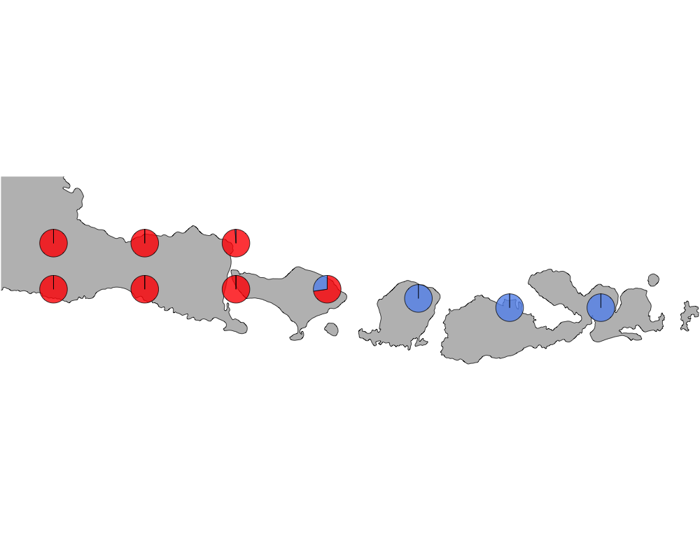
cutoff
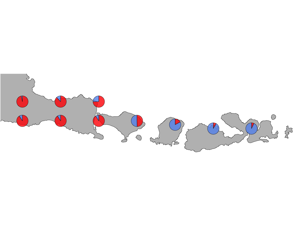
cut-off = 20

cutoff
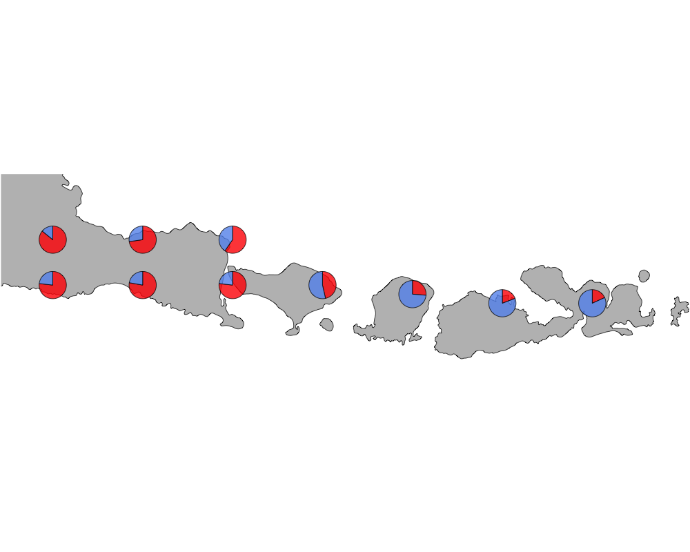
cut-off = 50

cutoff
cut-off = 70
cutoff
cut-off = 80

cutoff
cut-off = 90
cutoff
In summary, we see a distinction between species in Eastern and Western Indonesia going far far back.
SessionInfo
sessionInfo()## R version 3.4.4 (2018-03-15)
## Platform: x86_64-apple-darwin15.6.0 (64-bit)
## Running under: macOS Sierra 10.12.6
##
## Matrix products: default
## BLAS: /Library/Frameworks/R.framework/Versions/3.4/Resources/lib/libRblas.0.dylib
## LAPACK: /Library/Frameworks/R.framework/Versions/3.4/Resources/lib/libRlapack.dylib
##
## locale:
## [1] en_US.UTF-8/en_US.UTF-8/en_US.UTF-8/C/en_US.UTF-8/en_US.UTF-8
##
## attached base packages:
## [1] stats graphics grDevices utils datasets methods base
##
## other attached packages:
## [1] phytools_0.6-44 ape_5.0 ggthemes_3.4.0
## [4] scales_0.5.0.9000 mapplots_1.5 mapdata_2.2-6
## [7] maps_3.2.0 rgdal_1.2-16 gtools_3.5.0
## [10] rasterVis_0.41 latticeExtra_0.6-28 RColorBrewer_1.1-2
## [13] lattice_0.20-35 raster_2.6-7 sp_1.2-7
## [16] CountClust_1.5.1 ggplot2_2.2.1 methClust_0.1.0
##
## loaded via a namespace (and not attached):
## [1] viridisLite_0.3.0 splines_3.4.4
## [3] assertthat_0.2.0 expm_0.999-2
## [5] stats4_3.4.4 animation_2.5
## [7] yaml_2.1.18 slam_0.1-42
## [9] numDeriv_2016.8-1 pillar_1.1.0
## [11] backports_1.1.2 quadprog_1.5-5
## [13] limma_3.34.8 phangorn_2.3.1
## [15] digest_0.6.15 colorspace_1.3-2
## [17] picante_1.6-2 cowplot_0.9.2
## [19] htmltools_0.3.6 Matrix_1.2-12
## [21] plyr_1.8.4 pkgconfig_2.0.1
## [23] mvtnorm_1.0-6 combinat_0.0-8
## [25] tibble_1.4.2 mgcv_1.8-23
## [27] nnet_7.3-12 hexbin_1.27.1
## [29] lazyeval_0.2.1 mnormt_1.5-5
## [31] survival_2.41-3 magrittr_1.5
## [33] evaluate_0.10.1 msm_1.6.5
## [35] nlme_3.1-131.1 MASS_7.3-47
## [37] vegan_2.4-4 tools_3.4.4
## [39] stringr_1.3.0 munsell_0.4.3
## [41] plotrix_3.7 cluster_2.0.6
## [43] compiler_3.4.4 clusterGeneration_1.3.4
## [45] rlang_0.2.0 grid_3.4.4
## [47] igraph_1.1.2 rmarkdown_1.9
## [49] boot_1.3-20 gtable_0.2.0
## [51] flexmix_2.3-14 reshape2_1.4.3
## [53] zoo_1.8-0 knitr_1.20
## [55] fastmatch_1.1-0 rprojroot_1.3-2
## [57] maptpx_1.9-4 permute_0.9-4
## [59] modeltools_0.2-21 stringi_1.1.6
## [61] parallel_3.4.4 SQUAREM_2017.10-1
## [63] Rcpp_0.12.16 coda_0.19-1
## [65] scatterplot3d_0.3-40This R Markdown site was created with workflowr