Intro

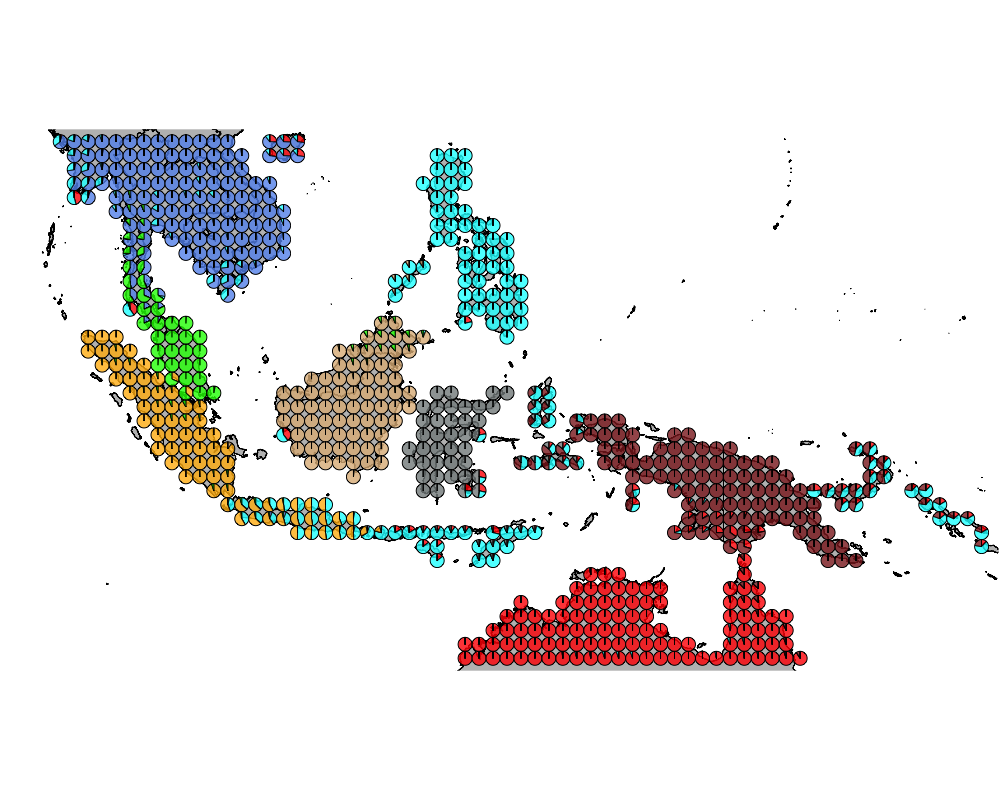
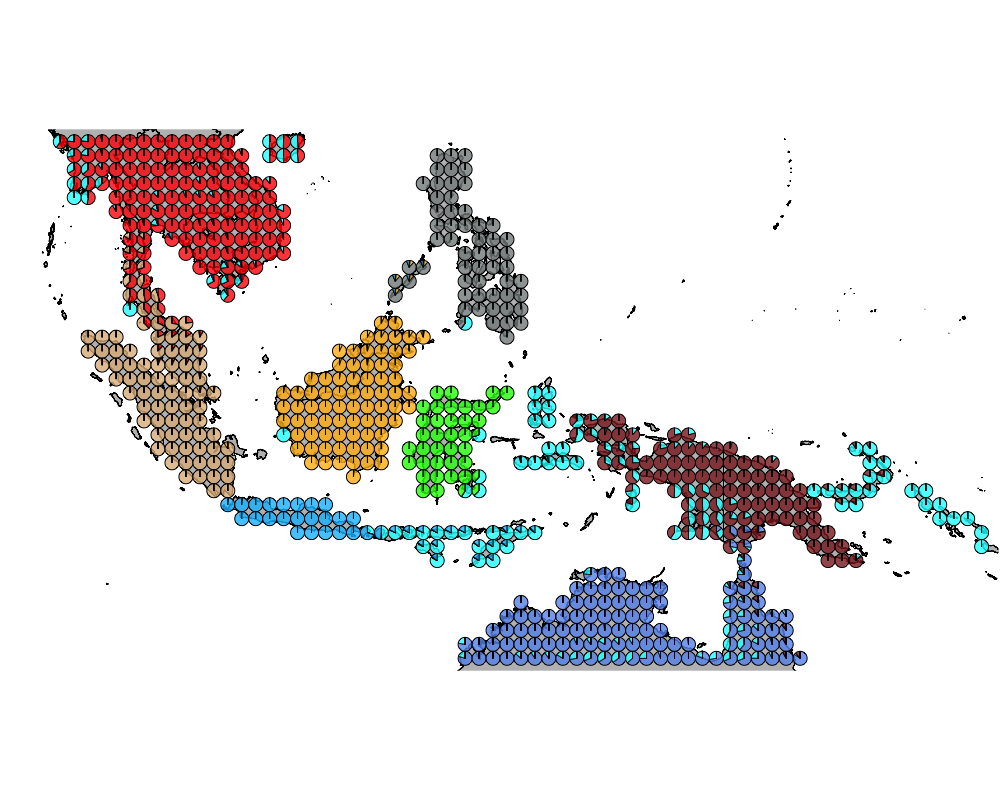
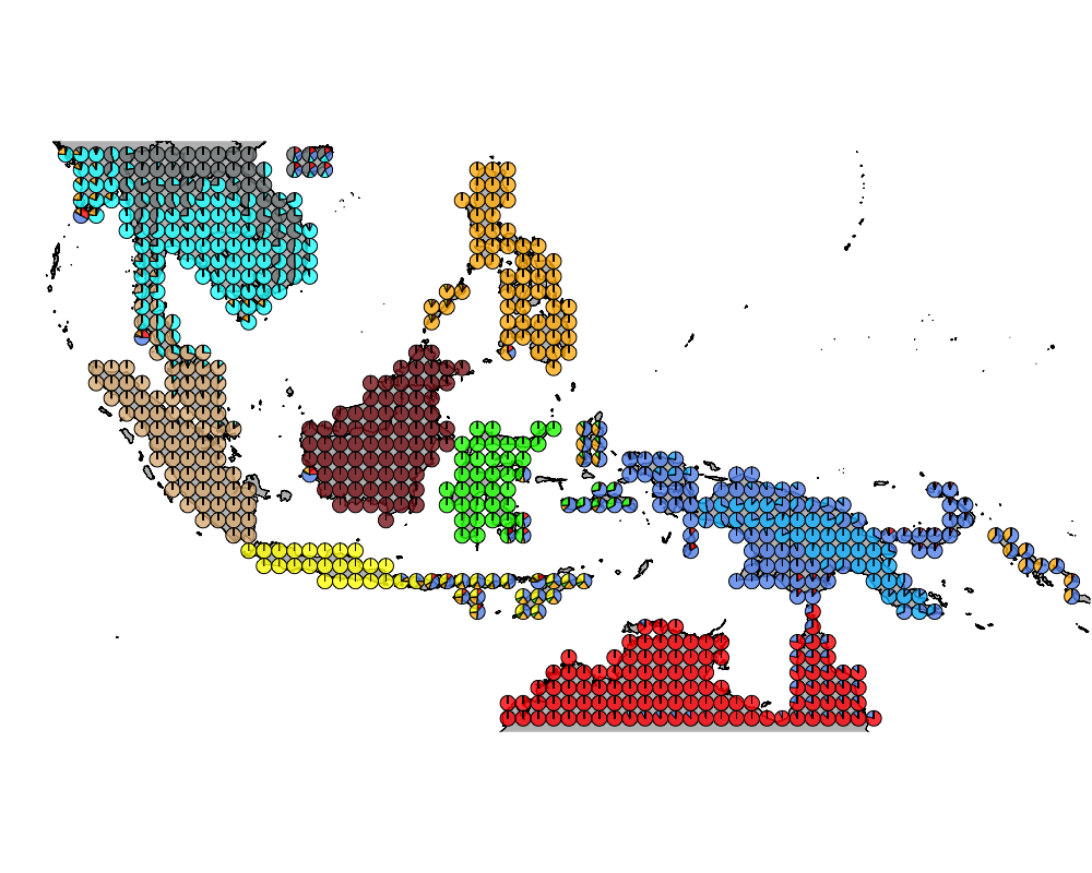
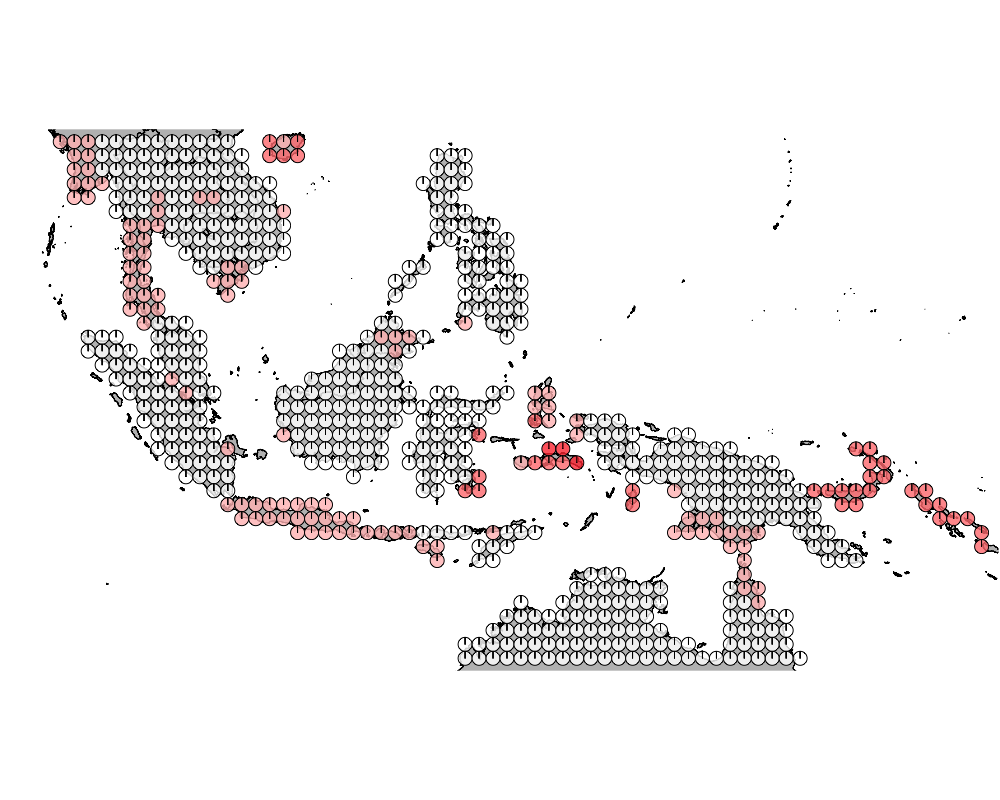
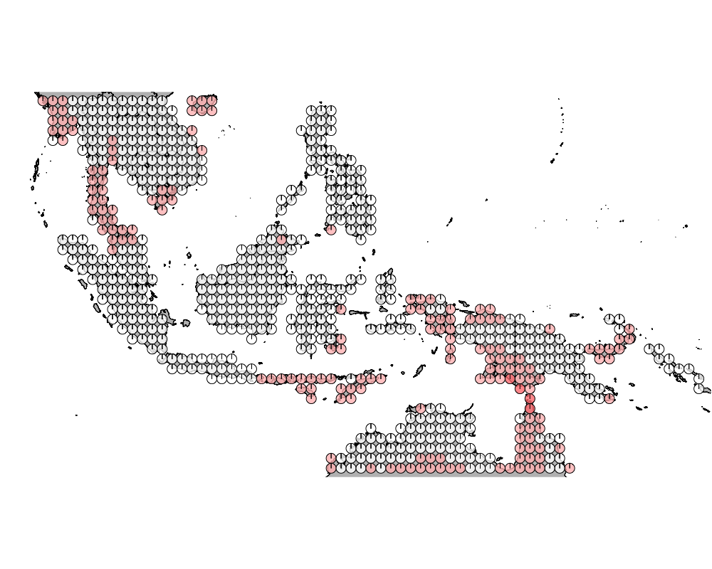
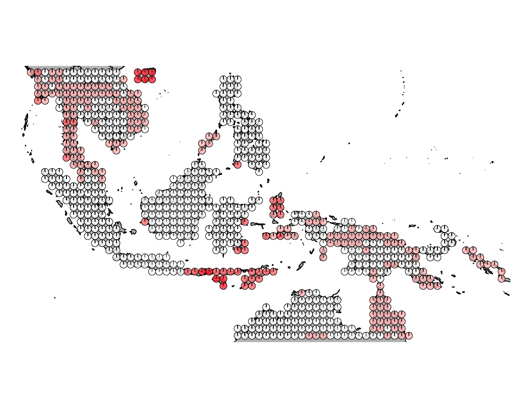
Here we look at those regions in Wallacea which has high admixture in terms of the presence of distinct communities of mammals.

Packages

library(methClust)
library(CountClust)
library(rasterVis)
library(gtools)
library(sp)
library(rgdal)
library(ggplot2)
library(maps)
library(mapdata)
library(mapplots)
library(scales)
library(ggthemes)

Load the data

Wallacea Region data

mamms <- get(load("../data/mammals_with_bats.rda"))
latlong_chars <- rownames(mamms)
latlong <- cbind.data.frame(as.numeric(sapply(latlong_chars, 
                              function(x) return(strsplit(x, "_")[[1]][1]))),
         as.numeric(sapply(latlong_chars, 
                           function(x) return(strsplit(x, "_")[[1]][2]))))

GoM model

topics_clust <- get(load("../output/methClust_wallacea_mammals_bats.rda"))

K = 8

K = 9

K = 10

Identifying number of mixed components

K = 8

topics <- topics_clust[[8]]
num_components <- apply(topics$omega, 1, function(x) return (length(which(x > 0.1))))
modelmat <- model.matrix(~as.factor(num_components)-1)

color = colorRampPalette(c("white", "red"))(5)
intensity <- 0.8
for(m in 1:1){
  png(filename=paste0("../docs/High_ADMIX_regions_mammals/high_admixture_K_8.png"),width = 1000, height = 800)
map("worldHires",
    ylim=c(-18,20), xlim=c(90,160), # Re-defines the latitude and longitude range
    col = "gray", fill=TRUE, mar=c(0.1,0.1,0.1,0.1))
lapply(1:dim(modelmat)[1], function(r)
  add.pie(z=as.integer(100*modelmat[r,]),
          x=latlong[r,1], y=latlong[r,2], labels=c("","",""),
          radius = 0.5,
          col=c(alpha(color[1],intensity),alpha(color[2],intensity),
                alpha(color[3], intensity), alpha(color[4], intensity),
                alpha(color[5], intensity))));
dev.off()
}

K = 9

topics <- topics_clust[[9]]
num_components <- apply(topics$omega, 1, function(x) return (length(which(x > 0.1))))
modelmat <- model.matrix(~as.factor(num_components)-1)

color = colorRampPalette(c("white", "red"))(5)
intensity <- 0.8
for(m in 1:1){
  png(filename=paste0("../docs/High_ADMIX_regions_mammals/high_admixture_K_9.png"),width = 1000, height = 800)
map("worldHires",
    ylim=c(-18,20), xlim=c(90,160), # Re-defines the latitude and longitude range
    col = "gray", fill=TRUE, mar=c(0.1,0.1,0.1,0.1))
lapply(1:dim(modelmat)[1], function(r)
  add.pie(z=as.integer(100*modelmat[r,]),
          x=latlong[r,1], y=latlong[r,2], labels=c("","",""),
          radius = 0.5,
          col=c(alpha(color[1],intensity),alpha(color[2],intensity),
                alpha(color[3], intensity), alpha(color[4], intensity),
                alpha(color[5], intensity))));
dev.off()
}

K = 10

topics <- topics_clust[[10]]
num_components <- apply(topics$omega, 1, function(x) return (length(which(x > 0.1))))
modelmat <- model.matrix(~as.factor(num_components)-1)

color = colorRampPalette(c("white", "red"))(5)
intensity <- 0.8
for(m in 1:1){
  png(filename=paste0("../docs/High_ADMIX_regions_mammals/high_admixture_K_10.png"),width = 1000, height = 800)
map("worldHires",
    ylim=c(-18,20), xlim=c(90,160), # Re-defines the latitude and longitude range
    col = "gray", fill=TRUE, mar=c(0.1,0.1,0.1,0.1))
lapply(1:dim(modelmat)[1], function(r)
  add.pie(z=as.integer(100*modelmat[r,]),
          x=latlong[r,1], y=latlong[r,2], labels=c("","",""),
          radius = 0.5,
          col=c(alpha(color[1],intensity),alpha(color[2],intensity),
                alpha(color[3], intensity), alpha(color[4], intensity),
                alpha(color[5], intensity))));
dev.off()
}

Visualization of high admix regions

K = 8

K = 9

geostructure10

K = 10

geostructure10

sessionInfo()

## R version 3.5.0 (2018-04-23)
## Platform: x86_64-apple-darwin15.6.0 (64-bit)
## Running under: macOS Sierra 10.12.6
## 
## Matrix products: default
## BLAS: /Library/Frameworks/R.framework/Versions/3.5/Resources/lib/libRblas.0.dylib
## LAPACK: /Library/Frameworks/R.framework/Versions/3.5/Resources/lib/libRlapack.dylib
## 
## locale:
## [1] en_US.UTF-8/en_US.UTF-8/en_US.UTF-8/C/en_US.UTF-8/en_US.UTF-8
## 
## attached base packages:
## [1] stats     graphics  grDevices utils     datasets  methods   base     
## 
## other attached packages:
##  [1] ggthemes_3.5.0      scales_0.5.0        mapplots_1.5       
##  [4] mapdata_2.3.0       maps_3.3.0          rgdal_1.2-20       
##  [7] gtools_3.5.0        rasterVis_0.44      latticeExtra_0.6-28
## [10] RColorBrewer_1.1-2  lattice_0.20-35     raster_2.6-7       
## [13] sp_1.2-7            CountClust_1.6.1    ggplot2_2.2.1      
## [16] methClust_0.1.0    
## 
## loaded via a namespace (and not attached):
##  [1] zoo_1.8-1         modeltools_0.2-21 slam_0.1-43      
##  [4] reshape2_1.4.3    colorspace_1.3-2  htmltools_0.3.6  
##  [7] stats4_3.5.0      viridisLite_0.3.0 yaml_2.1.19      
## [10] mgcv_1.8-23       rlang_0.2.0       hexbin_1.27.2    
## [13] pillar_1.2.2      plyr_1.8.4        stringr_1.3.1    
## [16] munsell_0.4.3     gtable_0.2.0      evaluate_0.10.1  
## [19] knitr_1.20        permute_0.9-4     flexmix_2.3-14   
## [22] parallel_3.5.0    Rcpp_0.12.17      backports_1.1.2  
## [25] limma_3.36.1      vegan_2.5-1       maptpx_1.9-5     
## [28] picante_1.7       digest_0.6.15     stringi_1.2.2    
## [31] cowplot_0.9.2     grid_3.5.0        rprojroot_1.3-2  
## [34] tools_3.5.0       magrittr_1.5      lazyeval_0.2.1   
## [37] tibble_1.4.2      cluster_2.0.7-1   ape_5.1          
## [40] MASS_7.3-49       Matrix_1.2-14     SQUAREM_2017.10-1
## [43] assertthat_0.2.0  rmarkdown_1.9     boot_1.3-20      
## [46] nnet_7.3-12       nlme_3.1-137      compiler_3.5.0

This R Markdown site was created with workflowr