High admixture regions in the Wallace region

Introduction

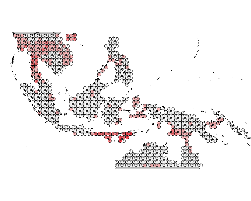
In this script, we look at the high admixture regions in Wallacea. High admixture is defined as having substantial memberships in many clusters. Usually each grid cell has substantial membership (say > 0.1) in one cluster - but some grid cells may have an admixing of the different communities of bird species and they will show high memberships in multiple clusters.

Packages

library(methClust)
library(CountClust)
library(rasterVis)
library(gtools)
library(sp)
library(rgdal)
library(ggplot2)
library(maps)
library(mapdata)
library(mapplots)
library(scales)
library(ggthemes)

Load the data

Wallacea Region data

birds <- get(load("../data/wallacea_birds.rda"))
latlong_chars_birds <- rownames(birds)
latlong <- cbind.data.frame(as.numeric(sapply(latlong_chars_birds, 
              function(x) return(strsplit(x, "_")[[1]][1]))),
         as.numeric(sapply(latlong_chars_birds, 
              function(x) return(strsplit(x, "_")[[1]][2]))))

GoM model

topics_clust <- get(load("../output/methClust_wallacea_birds.rda"))

ecoSTRUCTURE plot visualization

K = 8

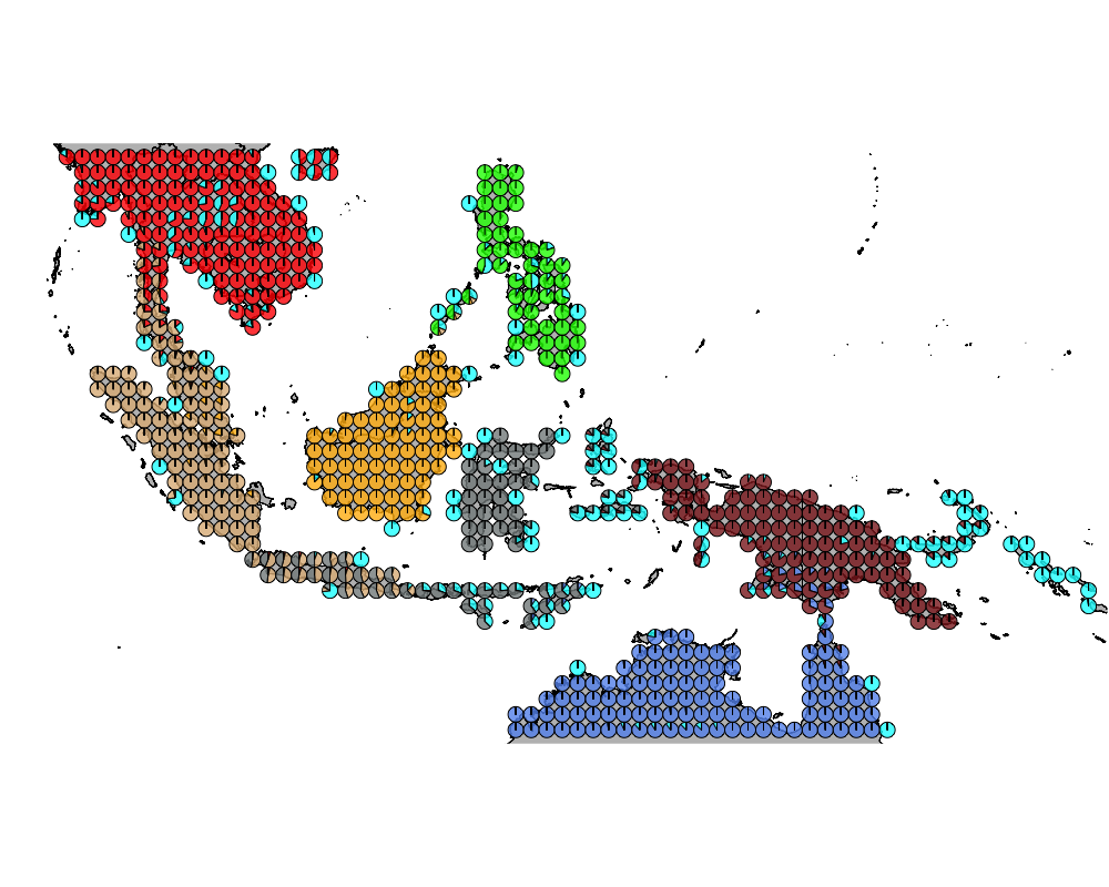
geostructure10

K = 9

geostructure10

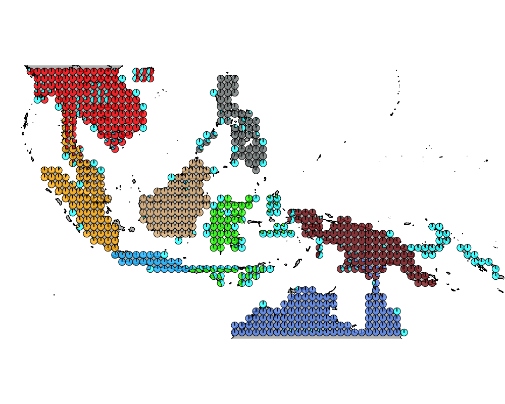
K = 10

geostructure10

Identifying number of mixed components

topics <- topics_clust[[8]]
num_components <- apply(topics$omega, 1, function(x) return (length(which(x > 0.1))))
modelmat <- model.matrix(~as.factor(num_components)-1)

color = colorRampPalette(c("white", "red"))(5)
intensity <- 0.8
for(m in 1:1){
  png(filename=paste0("../docs/High_ADMIX_regions_birds/high_admixture_K_8.png"),width = 1000, height = 800)
map("worldHires",
    ylim=c(-18,20), xlim=c(90,160), # Re-defines the latitude and longitude range
    col = "gray", fill=TRUE, mar=c(0.1,0.1,0.1,0.1))
lapply(1:dim(modelmat)[1], function(r)
  add.pie(z=as.integer(100*modelmat[r,]),
          x=latlong[r,1], y=latlong[r,2], labels=c("","",""),
          radius = 0.5,
          col=c(alpha(color[1],intensity),alpha(color[2],intensity),
                alpha(color[3], intensity), alpha(color[4], intensity),
                alpha(color[5], intensity))));
dev.off()
}

topics <- topics_clust[[9]]
num_components <- apply(topics$omega, 1, function(x) return (length(which(x > 0.1))))
modelmat <- model.matrix(~as.factor(num_components)-1)

color = colorRampPalette(c("white", "red"))(5)
intensity <- 0.8
for(m in 1:1){
  png(filename=paste0("../docs/High_ADMIX_regions_birds/high_admixture_K_9.png"),width = 1000, height = 800)
map("worldHires",
    ylim=c(-18,20), xlim=c(90,160), # Re-defines the latitude and longitude range
    col = "gray", fill=TRUE, mar=c(0.1,0.1,0.1,0.1))
lapply(1:dim(modelmat)[1], function(r)
  add.pie(z=as.integer(100*modelmat[r,]),
          x=latlong[r,1], y=latlong[r,2], labels=c("","",""),
          radius = 0.5,
          col=c(alpha(color[1],intensity),alpha(color[2],intensity),
                alpha(color[3], intensity), alpha(color[4], intensity),
                alpha(color[5], intensity))));
dev.off()
}

topics <- topics_clust[[10]]
num_components <- apply(topics$omega, 1, function(x) return (length(which(x > 0.1))))
modelmat <- model.matrix(~as.factor(num_components)-1)

color = colorRampPalette(c("white", "red"))(5)
intensity <- 0.8
for(m in 1:1){
  png(filename=paste0("../docs/High_ADMIX_regions_birds/high_admixture_K_10.png"),width = 1000, height = 800)
map("worldHires",
    ylim=c(-18,20), xlim=c(90,160), # Re-defines the latitude and longitude range
    col = "gray", fill=TRUE, mar=c(0.1,0.1,0.1,0.1))
lapply(1:dim(modelmat)[1], function(r)
  add.pie(z=as.integer(100*modelmat[r,]),
          x=latlong[r,1], y=latlong[r,2], labels=c("","",""),
          radius = 0.5,
          col=c(alpha(color[1],intensity),alpha(color[2],intensity),
                alpha(color[3], intensity), alpha(color[4], intensity),
                alpha(color[5], intensity))));
dev.off()
}

Visualization of high admix regions

K = 8

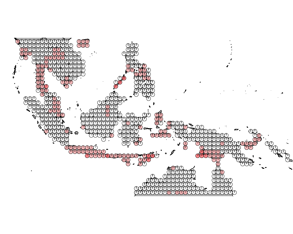
geostructure10

K = 9

geostructure10

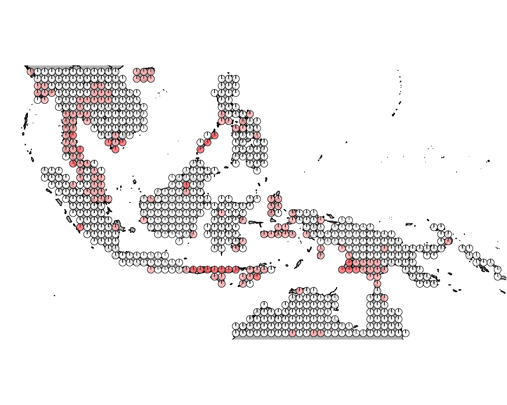
K = 10

geostructure10

Overall we see that the strips of islnads in the Wallacea region are highly admixed.

SessionInfo

sessionInfo()

## R version 3.5.0 (2018-04-23)
## Platform: x86_64-apple-darwin15.6.0 (64-bit)
## Running under: macOS Sierra 10.12.6
## 
## Matrix products: default
## BLAS: /Library/Frameworks/R.framework/Versions/3.5/Resources/lib/libRblas.0.dylib
## LAPACK: /Library/Frameworks/R.framework/Versions/3.5/Resources/lib/libRlapack.dylib
## 
## locale:
## [1] en_US.UTF-8/en_US.UTF-8/en_US.UTF-8/C/en_US.UTF-8/en_US.UTF-8
## 
## attached base packages:
## [1] stats     graphics  grDevices utils     datasets  methods   base     
## 
## other attached packages:
##  [1] ggthemes_3.5.0      scales_0.5.0        mapplots_1.5       
##  [4] mapdata_2.3.0       maps_3.3.0          rgdal_1.2-20       
##  [7] gtools_3.5.0        rasterVis_0.44      latticeExtra_0.6-28
## [10] RColorBrewer_1.1-2  lattice_0.20-35     raster_2.6-7       
## [13] sp_1.2-7            CountClust_1.6.1    ggplot2_2.2.1      
## [16] methClust_0.1.0    
## 
## loaded via a namespace (and not attached):
##  [1] zoo_1.8-1         modeltools_0.2-21 slam_0.1-43      
##  [4] reshape2_1.4.3    colorspace_1.3-2  htmltools_0.3.6  
##  [7] stats4_3.5.0      viridisLite_0.3.0 yaml_2.1.19      
## [10] mgcv_1.8-23       rlang_0.2.0       hexbin_1.27.2    
## [13] pillar_1.2.2      plyr_1.8.4        stringr_1.3.1    
## [16] munsell_0.4.3     gtable_0.2.0      evaluate_0.10.1  
## [19] knitr_1.20        permute_0.9-4     flexmix_2.3-14   
## [22] parallel_3.5.0    Rcpp_0.12.17      backports_1.1.2  
## [25] limma_3.36.1      vegan_2.5-1       maptpx_1.9-5     
## [28] picante_1.7       digest_0.6.15     stringi_1.2.2    
## [31] cowplot_0.9.2     grid_3.5.0        rprojroot_1.3-2  
## [34] tools_3.5.0       magrittr_1.5      lazyeval_0.2.1   
## [37] tibble_1.4.2      cluster_2.0.7-1   ape_5.1          
## [40] MASS_7.3-49       Matrix_1.2-14     SQUAREM_2017.10-1
## [43] assertthat_0.2.0  rmarkdown_1.9     boot_1.3-20      
## [46] nnet_7.3-12       nlme_3.1-137      compiler_3.5.0