Wallace Line Driving Birds

Data Processing + driving birds extraction

latlong <- get(load("../data/LatLongCells_frame.rda"))

world_map <- map_data("world")
world_map <- world_map[world_map$region != "Antarctica",] # intercourse antarctica

world_map <- world_map[world_map$long > 90 & world_map$long < 160, ]
world_map <- world_map[world_map$lat > -18 & world_map$lat < 20, ]


p <- ggplot() + coord_fixed() +
  xlab("") + ylab("")

#Add map to base plot
base_world_messy <- p + geom_polygon(data=world_map, aes(x=long, y=lat, group=group), colour="light green", fill="light green")

cleanup <- 
  theme(panel.grid.major = element_blank(), panel.grid.minor = element_blank(), 
        panel.background = element_rect(fill = 'white', colour = 'white'), 
        axis.line = element_line(colour = "white"), legend.position="none",
        axis.ticks=element_blank(), axis.text.x=element_blank(),
        axis.text.y=element_blank())

base_world <- base_world_messy + cleanup

base_world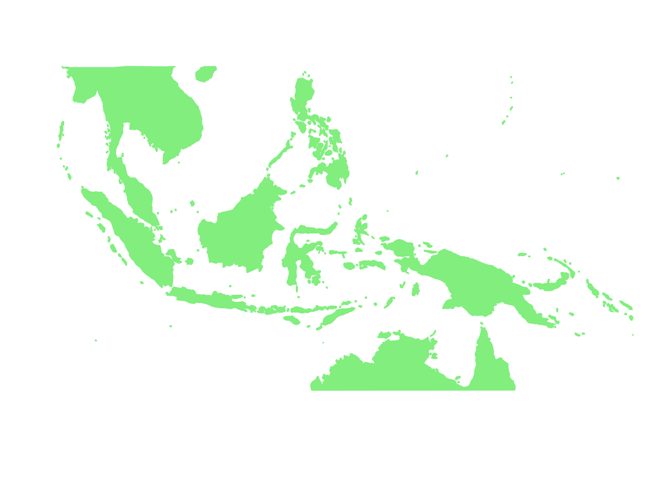

latlong <- get(load("../data/LatLongCells_frame.rda"))

idx1 <- which(latlong[,2] > -18 & latlong[,2] < 20)
idx2 <- which(latlong[,1] > 90 & latlong[,1] < 160)
idx <- intersect(idx1, idx2)
length(idx)

## [1] 703

latlong2 <- latlong[idx,]

birds_pa_data <- readRDS("../data/birds_presab_land_breeding_counts.rds")
birds_pa_data_2 <- birds_pa_data[idx, ]
birds_pa_data_3 <- birds_pa_data_2[, which(colSums(birds_pa_data_2)!=0)]

Names of driving bird species

topics <- get(load("../output/Wallacea/methClust_2.rda"))

second_topic_scores <- topics$freq[,2] - topics$freq[,1]
first_topic_scores <- topics$freq[,1] - topics$freq[,2]

Second topic birds

names(second_topic_scores)[order(second_topic_scores, decreasing = TRUE)[1:10]]

##  [1] "Amaurornis phoenicurus"    "Centropus bengalensis"    
##  [3] "Cypsiurus balasiensis"     "Gallinula chloropus"      
##  [5] "Hypothymis azurea"         "Eudynamys scolopaceus"    
##  [7] "Spilopelia chinensis"      "Aegithina tiphia"         
##  [9] "Anthracoceros albirostris" "Irena puella"

First topic birds

names(first_topic_scores)[order(first_topic_scores, decreasing = TRUE)[1:10]]

##  [1] "Anas gracilis"          "Eudynamys orientalis"  
##  [3] "Nycticorax caledonicus" "Anas superciliosa"     
##  [5] "Rhipidura leucophrys"   "Coracina papuensis"    
##  [7] "Corvus orru"            "Megalurus timoriensis" 
##  [9] "Rhipidura rufiventris"  "Cacatua galerita"

Patterns of presence absence of driving bird species

PlotAssemblageIdx <- function(idx){
  dat <- cbind.data.frame(latlong2, birds_pa_data_3[,idx])
colnames(dat) <- c("Latitude", "Longitude", "Value")
map_data_coloured <- 
  base_world +
  geom_point(data=dat, 
             aes(x=Latitude, y=Longitude, colour=Value), size=0.5) +
  scale_colour_gradient(low = "white", high = "black") 

map_data_coloured
}

par(mfrow = c(5,2))
for(m in 1:10){
  PlotAssemblageIdx(order(second_topic_scores, decreasing = TRUE)[m])
}

par(mfrow = c(5,2))
PlotAssemblageIdx(order(second_topic_scores, decreasing = TRUE)[1])

PlotAssemblageIdx(order(second_topic_scores, decreasing = TRUE)[2])

PlotAssemblageIdx(order(second_topic_scores, decreasing = TRUE)[3])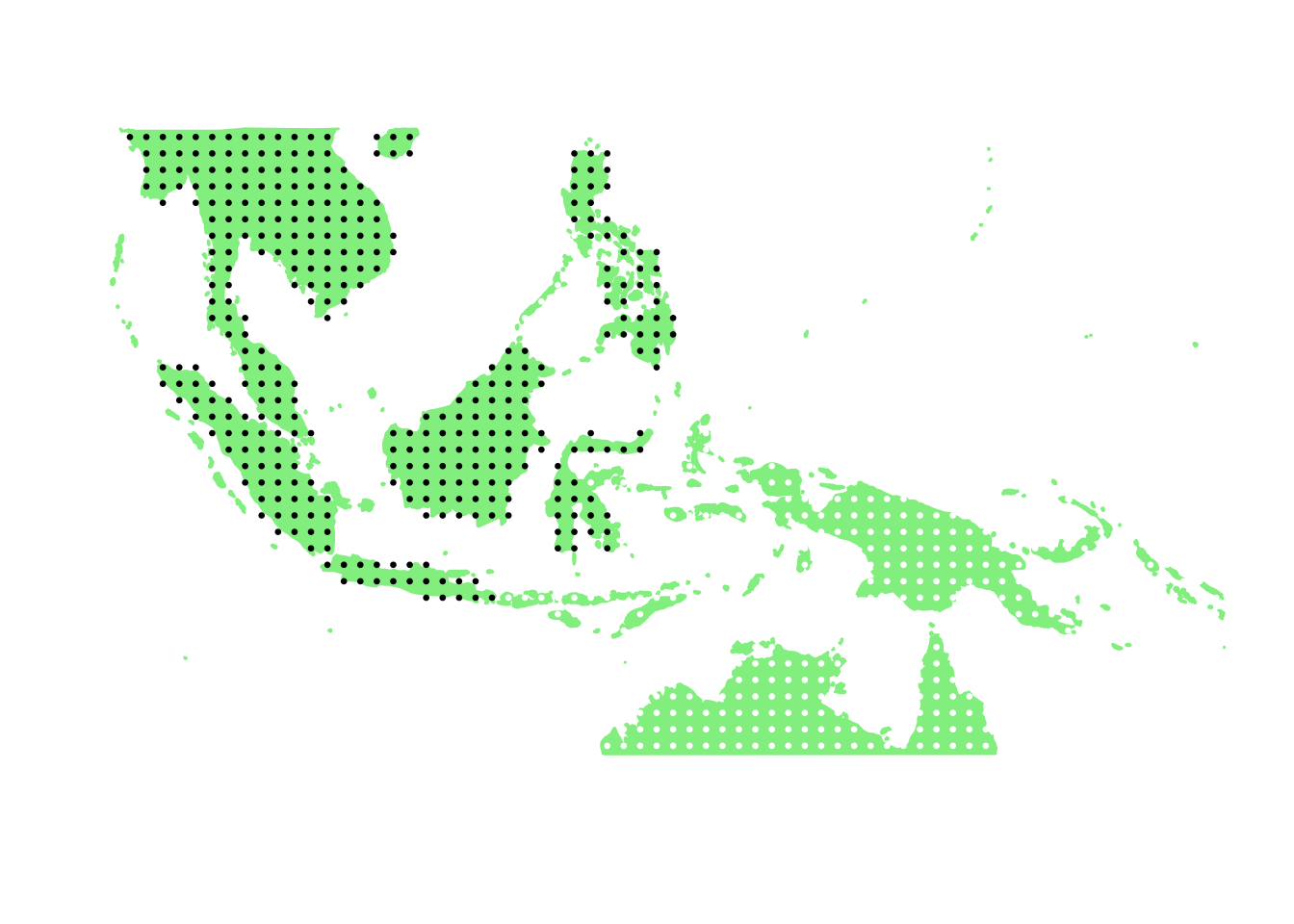

PlotAssemblageIdx(order(second_topic_scores, decreasing = TRUE)[4])

PlotAssemblageIdx(order(second_topic_scores, decreasing = TRUE)[5])

PlotAssemblageIdx(order(second_topic_scores, decreasing = TRUE)[6])

PlotAssemblageIdx(order(second_topic_scores, decreasing = TRUE)[7])

PlotAssemblageIdx(order(second_topic_scores, decreasing = TRUE)[8])

PlotAssemblageIdx(order(second_topic_scores, decreasing = TRUE)[9])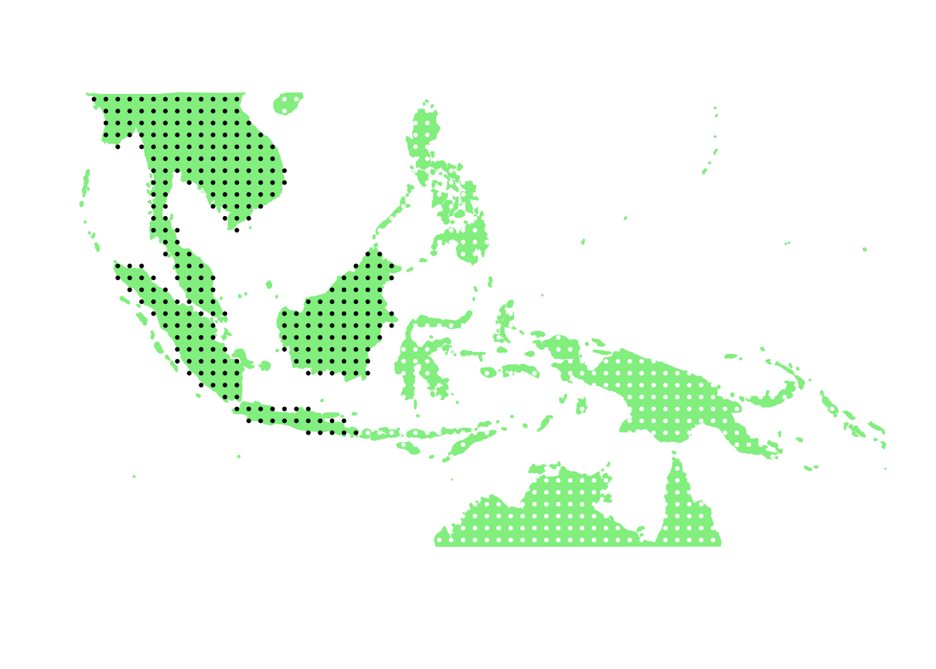

PlotAssemblageIdx(order(second_topic_scores, decreasing = TRUE)[10])

par(mfrow = c(5,2))
PlotAssemblageIdx(order(first_topic_scores, decreasing = TRUE)[1])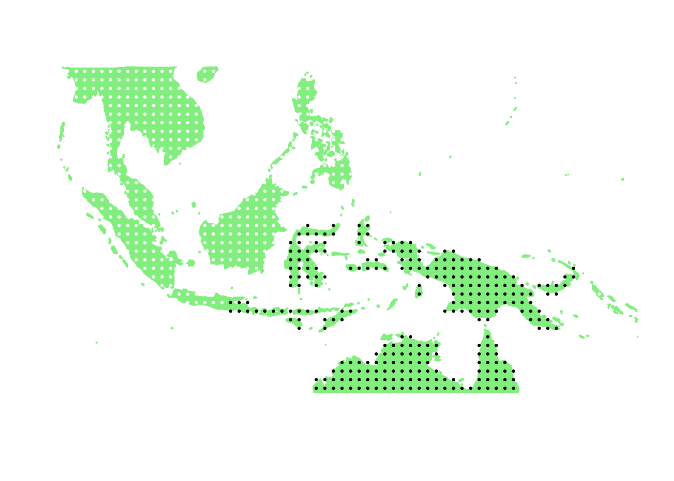

PlotAssemblageIdx(order(first_topic_scores, decreasing = TRUE)[2])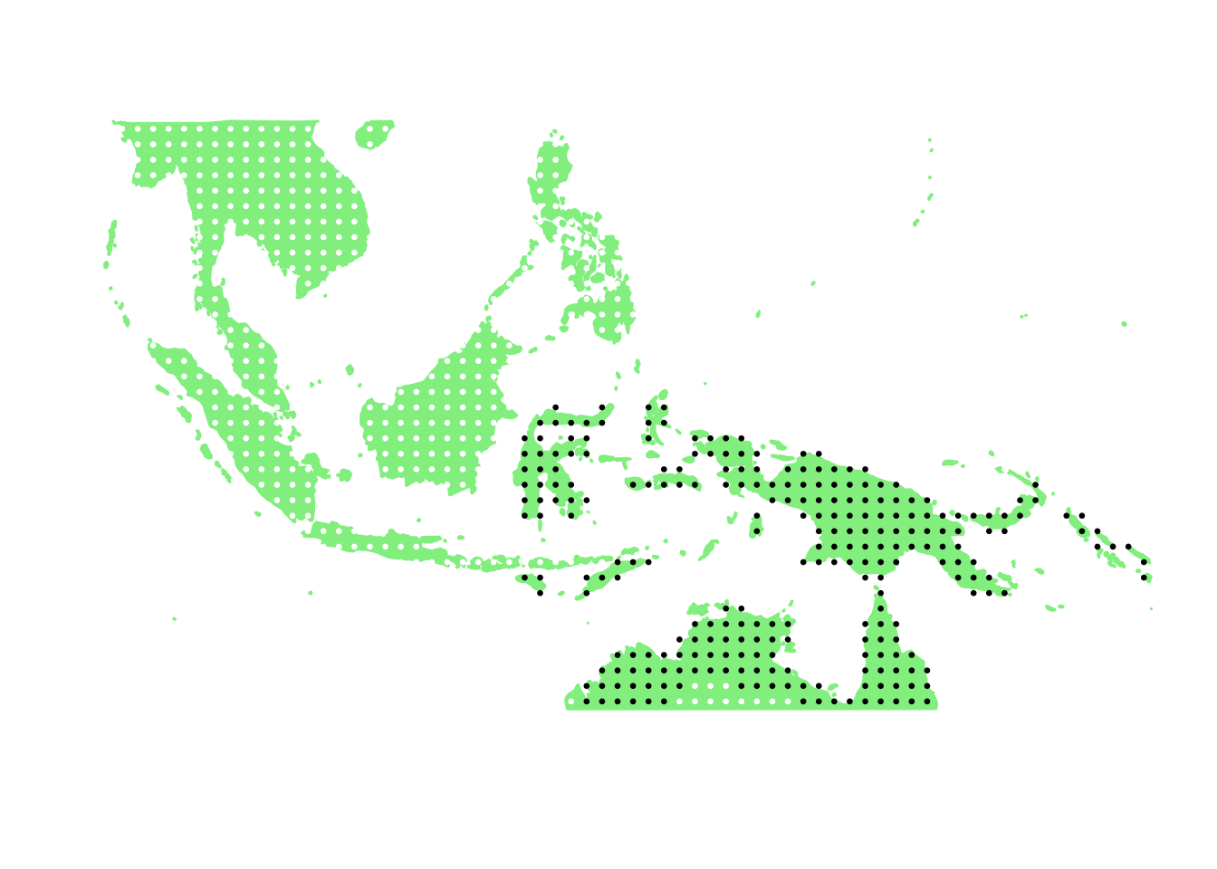

PlotAssemblageIdx(order(first_topic_scores, decreasing = TRUE)[3])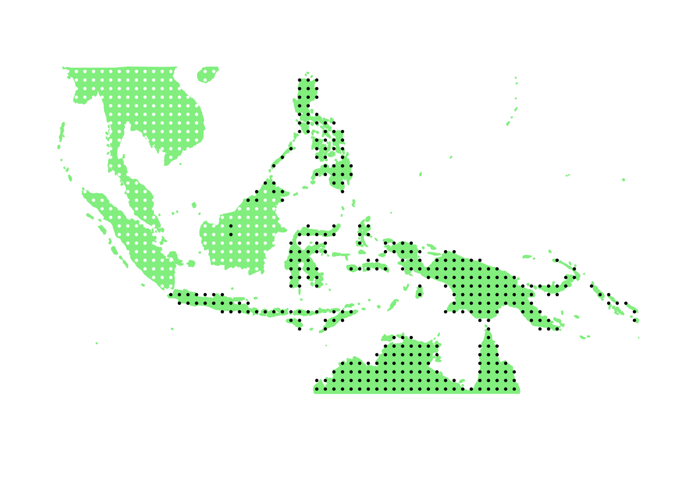

PlotAssemblageIdx(order(first_topic_scores, decreasing = TRUE)[4])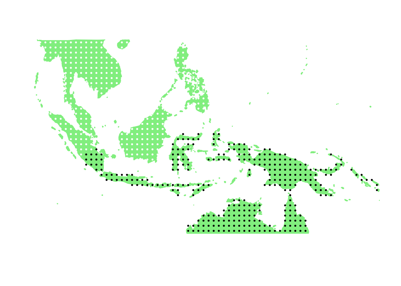

PlotAssemblageIdx(order(first_topic_scores, decreasing = TRUE)[5])

PlotAssemblageIdx(order(first_topic_scores, decreasing = TRUE)[6])

PlotAssemblageIdx(order(first_topic_scores, decreasing = TRUE)[7])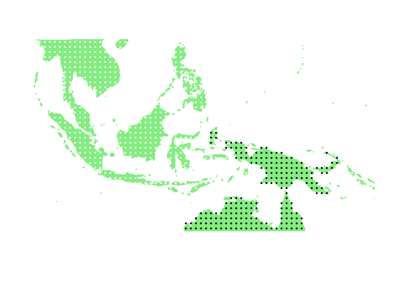

PlotAssemblageIdx(order(first_topic_scores, decreasing = TRUE)[8])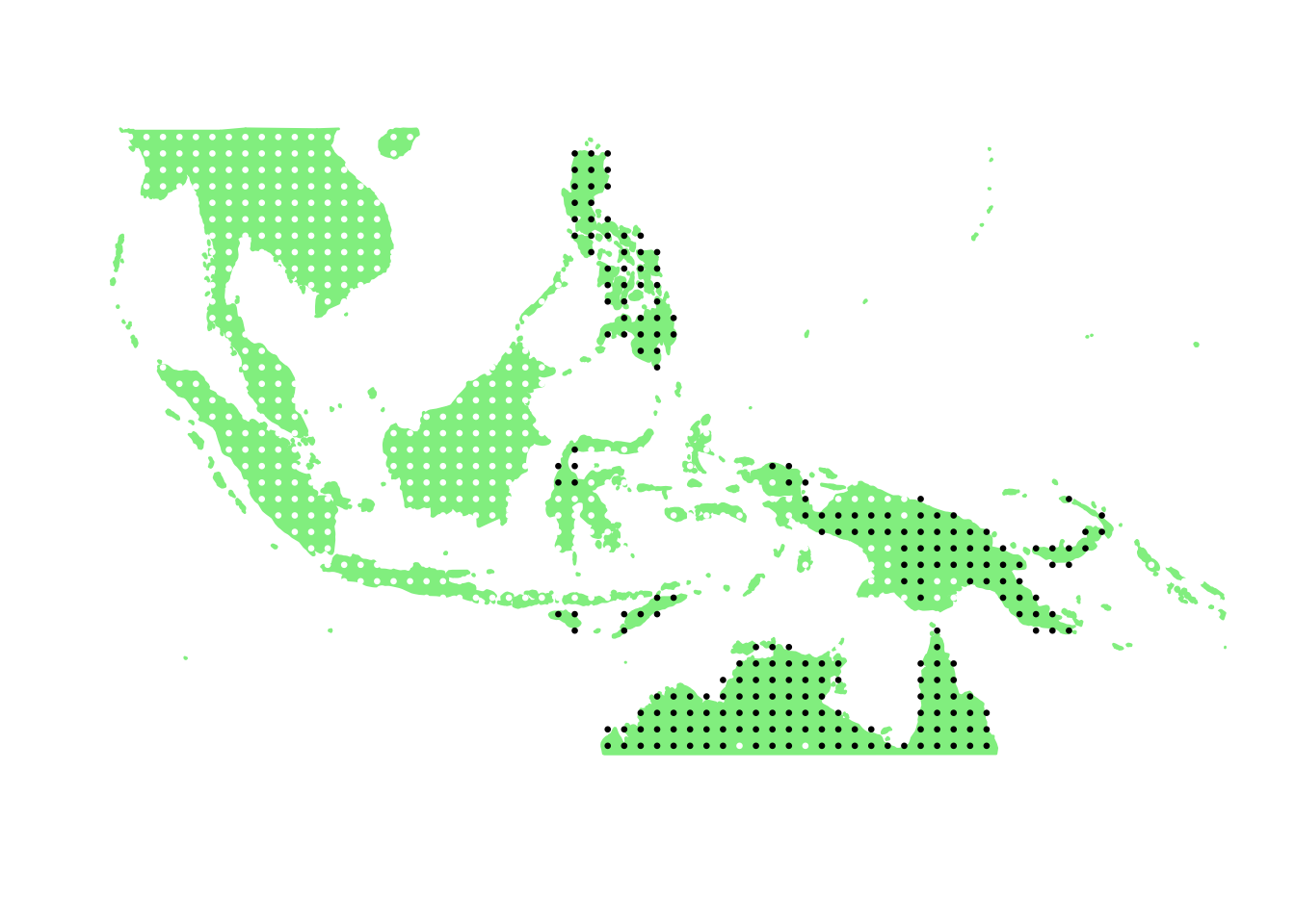

PlotAssemblageIdx(order(first_topic_scores, decreasing = TRUE)[9])

PlotAssemblageIdx(order(first_topic_scores, decreasing = TRUE)[10])