methClust on hCh data
Kushal K Dey
11/18/2017
Load packages
library(methClust)
library(CountClust)
## Loading required package: ggplot2library(ggplot2)
library(Seurat)## Loading required package: cowplot##
## Attaching package: 'cowplot'## The following object is masked from 'package:ggplot2':
##
## ggsave## Loading required package: Matrixlibrary(Rtsne)
library(mapplots)Load the methylation and non-methylation counts data
meth <- read.table("../data/meth.txt", header = TRUE)
unmeth <- read.table("../data/unmeth_w_zero.txt", header = TRUE)
rownames(meth) <- paste0("Bins_", 1:dim(meth)[1])
rownames(unmeth) <- paste0("Bins_", 1:dim(unmeth)[1])
logit_vals <- t(log((meth+0.01)/(meth + unmeth + 0.02)))out <- Rtsne(logit_vals, dims = 2)
save(out, file = "../output/tsne_hch.rda")out <- get(load("../output/tsne_hch.rda"))
tsne_proj <- out$YLoad the list of methClust outputs from \(K=2\) to \(K=6\).
topic_clus <- list()
topic_clus[[1]] <- get(load("../output/methclust_hch_k_2.rda"))
topic_clus[[2]] <- get(load("../output/methclust_hch_k_3.rda"))
topic_clus[[3]] <- get(load("../output/methclust_hch_k_4.rda"))
topic_clus[[4]] <- get(load("../output/methclust_hch_k_5.rda"))
topic_clus[[5]] <- get(load("../output/methclust_hch_k_6.rda"))
t-SNE projections + Hard clustering from methClust
labels2 <- as.factor(apply(topic_clus[[1]]$omega, 1, function(x) return(which.max(x))))
labels3 <- as.factor(apply(topic_clus[[2]]$omega, 1, function(x) return(which.max(x))))
labels4 <- as.factor(apply(topic_clus[[3]]$omega, 1, function(x) return(which.max(x))))
labels5 <- as.factor(apply(topic_clus[[4]]$omega, 1, function(x) return(which.max(x))))
labels6 <- as.factor(apply(topic_clus[[5]]$omega, 1, function(x) return(which.max(x))))

data_ggplot <- data.frame(labels2 = labels2,
                          labels3 = labels3,
                          labels4 = labels4,
                          labels5 = labels5,
                          labels6 = labels6,
                          tSNE_1 = tsne_proj[, 1],
                          tSNE_2 = tsne_proj[, 2])
library(ggplot2)
plot1 <- ggplot(data_ggplot) + theme(panel.background = element_rect(colour = "black", size = 1),
                                     panel.grid.major = element_blank(),
                                     panel.grid.minor = element_blank(),
                                     axis.text.y = element_blank(),
                                     axis.text.x = element_blank(),
                                     axis.ticks = element_blank(),
                                     legend.text = element_text(size = 15)) + geom_point(aes(x = tSNE_1, y = tSNE_2, color = labels2), size = 0.5) + labs(x = 'tSNE 1', y = 'tSNE 2', title = '') + scale_color_discrete('')

plot2 <- ggplot(data_ggplot) + theme(panel.background = element_rect(colour = "black", size = 1),
                                     panel.grid.major = element_blank(),
                                     panel.grid.minor = element_blank(),
                                     axis.text.y = element_blank(),
                                     axis.text.x = element_blank(),
                                     axis.ticks = element_blank(),
                                     legend.text = element_text(size = 15)) + geom_point(aes(x = tSNE_1, y = tSNE_2, color = labels3), size = 0.5) + labs(x = 'tSNE 1', y = 'tSNE 2', title = '') + scale_color_discrete('')

plot3 <- ggplot(data_ggplot) + theme(panel.background = element_rect(colour = "black", size = 1),
                                     panel.grid.major = element_blank(),
                                     panel.grid.minor = element_blank(),
                                     axis.text.y = element_blank(),
                                     axis.text.x = element_blank(),
                                     axis.ticks = element_blank(),
                                     legend.text = element_text(size = 15)) + geom_point(aes(x = tSNE_1, y = tSNE_2, color = labels4), size = 0.5) + labs(x = 'tSNE 1', y = 'tSNE 2', title = '') + scale_color_discrete('')

plot4 <- ggplot(data_ggplot) + theme(panel.background = element_rect(colour = "black", size = 1),
                                     panel.grid.major = element_blank(),
                                     panel.grid.minor = element_blank(),
                                     axis.text.y = element_blank(),
                                     axis.text.x = element_blank(),
                                     axis.ticks = element_blank(),
                                     legend.text = element_text(size = 15)) + geom_point(aes(x = tSNE_1, y = tSNE_2, color = labels5), size = 0.5) + labs(x = 'tSNE 1', y = 'tSNE 2', title = '') + scale_color_discrete('')

plot5 <- ggplot(data_ggplot) + theme(panel.background = element_rect(colour = "black", size = 1),
                                     panel.grid.major = element_blank(),
                                     panel.grid.minor = element_blank(),
                                     axis.text.y = element_blank(),
                                     axis.text.x = element_blank(),
                                     axis.ticks = element_blank(),
                                     legend.text = element_text(size = 15)) + geom_point(aes(x = tSNE_1, y = tSNE_2, color = labels6), size = 0.5) + labs(x = 'tSNE 1', y = 'tSNE 2', title = '') + scale_color_discrete('')

plot_grid(plot1, plot2, plot3, plot4, plot5, ncol = 2, align = 'v')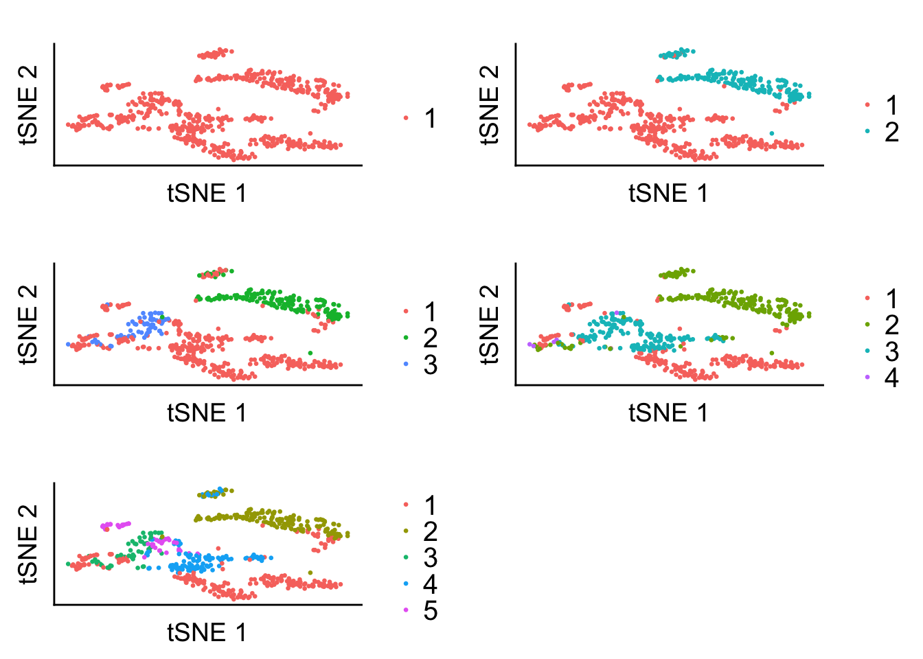
K-means Structure Plot
set.seed (100)
out <- kmeans(tsne_proj, centers = 10)
labels <- as.factor(out$cluster)
data_ggplot <- data.frame(labels = labels,
tSNE_1 = tsne_proj[, 1],
tSNE_2 = tsne_proj[, 2])
library(ggplot2)
plot1 <- ggplot(data_ggplot) + theme(panel.background = element_rect(colour = "black", size = 1),
panel.grid.major = element_blank(),
panel.grid.minor = element_blank(),
axis.text.y = element_blank(),
axis.text.x = element_blank(),
axis.ticks = element_blank(),
legend.text = element_text(size = 15)) + geom_point(aes(x = tSNE_1, y = tSNE_2, color = labels), size = 0.5) + labs(x = 'tSNE 1', y = 'tSNE 2', title = '') + scale_color_discrete('')
plot1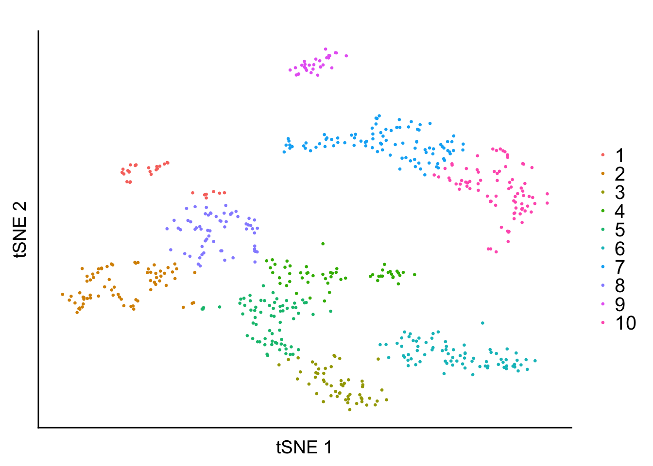
methClust Structure Plot
PlotmethClust <- function(topic_clus, fac){
  omega <- topic_clus$omega

  annotation <- data.frame(
    sample_id = paste0("X", 1:length(fac)),
    tissue_label = fac );

  rownames(omega) <- annotation$sample_id;

  StructureGGplot(omega = omega,
                  annotation = annotation,
                  palette = RColorBrewer::brewer.pal(8, "Accent"),
                  yaxis_label = "Types",
                  order_sample = TRUE,
                  axis_tick = list(axis_ticks_length = .1,
                                   axis_ticks_lwd_y = .1,
                                   axis_ticks_lwd_x = .1,
                                   axis_label_size = 7,
                                   axis_label_face = "bold"))
}
PlotmethClust(topic_clus[[1]], factor(labels, c(6, 3, 5, 4, 8, 1, 2, 10, 7, 9)))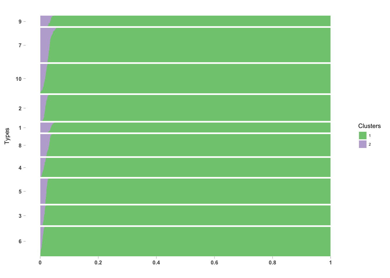
PlotmethClust(topic_clus[[2]], factor(labels, c(6, 3, 5, 4, 8, 1, 2, 10, 7, 9)))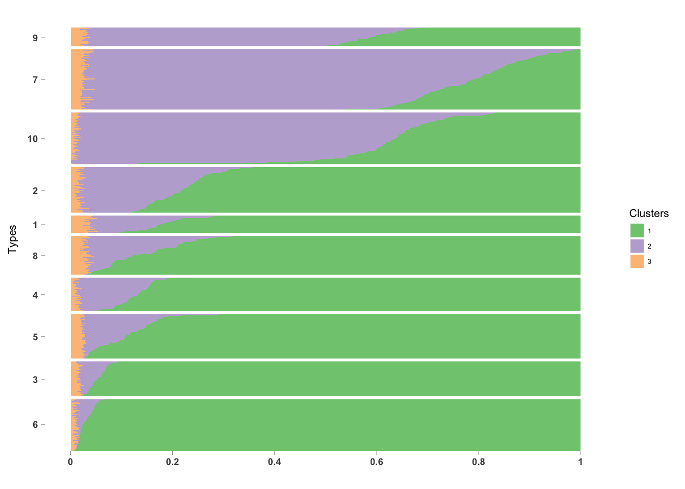
PlotmethClust(topic_clus[[3]], factor(labels, c(6, 3, 5, 4, 8, 1, 2, 10, 7, 9)))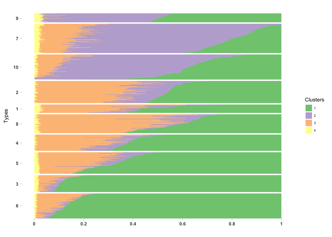
PlotmethClust(topic_clus[[4]], factor(labels, c(6, 3, 5, 4, 8, 1, 2, 10, 7, 9)))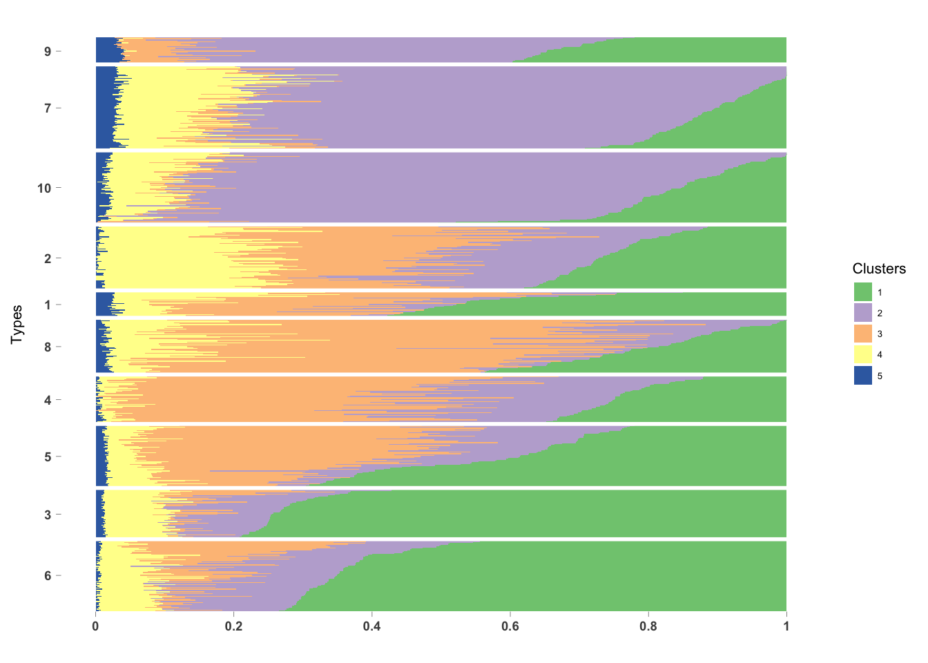
PlotmethClust(topic_clus[[5]], factor(labels, c(6, 3, 5, 4, 8, 1, 2, 10, 7, 9)))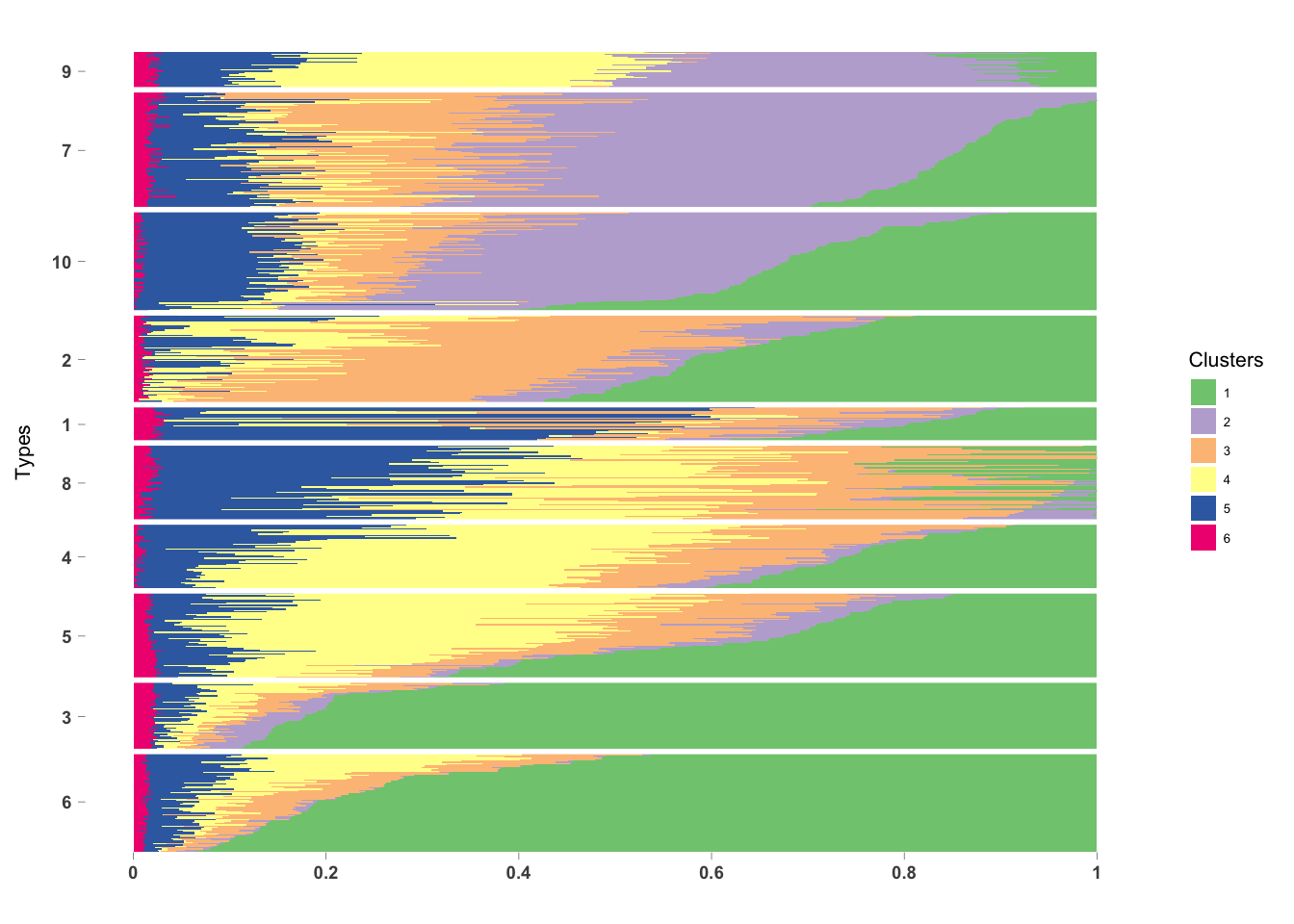
Cluster Profiles (K=3)
dim(topic_clus[[2]]$freq)## [1] 12905 3freq <- topic_clus[[2]]$freq
par(mfrow=c(2,2))
plot(freq[,1] - median(freq[,1]), col= "red", ylab = "freq", xlab = "bins")
plot(freq[,2] - median(freq[,2]), col= "red", ylab = "freq", xlab = "bins")
plot(freq[,3] - median(freq[,3]), col= "red", ylab = "freq", xlab = "bins")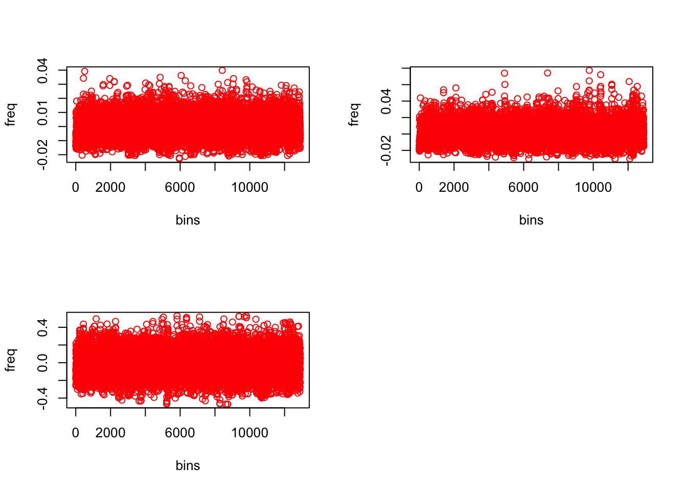
This R Markdown site was created with workflowr