methClust applications (0/1 scale) - Birds data
Kushal K Dey
12/2/2017
methClust is designed as a generic Binomial Grade of Membership model implementing software. A specific setting includes when the data is Bernoulli - that is observed versus unoberved. An example of such a setting is the presence-absence matrix from the bird abundance data.
Loading Birds Abundance Data
library(ecostructure)
library(methClust)
data <- get(load(system.file("extdata", "HimalayanBirdsData.rda",
package = "ecostructure")))
taxonomic_counts <- t(exprs(data))source("../../methClust/R/meth_topics.R")
source("../../methClust/R/meth_tpx.R")
source("../../methClust/R/meth_count.R")
library(slam)Presence absence Data
presence_absence <- taxonomic_counts
presence_absence[presence_absence > 0] = 1
absence_presence <- 1 - presence_absence
Application of methClust
apply methClust with the presence_absence matrix as analog to the methylation matrix and absence_presence matrix as analog to the unmethylation matrix.
topics_list <- list()

for(n in 1:100){
set.seed(100+n)
topics_list[[n]] <- meth_topics(presence_absence, absence_presence,
                      K=2, tol = 1, use_squarem = FALSE, NUM_INDICES_START = 10)
}
##
## Estimating on a 38 samples collection.
## log posterior increase: 6075.2, 6, 4.1, 17.2, 6.1, 8.4, 1.1, 5, 2.4, done.
##
## Estimating on a 38 samples collection.
## log posterior increase: 8360.4, done.
##
## Estimating on a 38 samples collection.
## log posterior increase: 9027.5, 2.8, 0.7, done.
##
## Estimating on a 38 samples collection.
## log posterior increase: 7844.2, done.
##
## Estimating on a 38 samples collection.
## log posterior increase: 7668.7, 1.7, done.
##
## Estimating on a 38 samples collection.
## log posterior increase: 7031.1, 4.4, 3.3, 9.3, 4.7, done.
##
## Estimating on a 38 samples collection.
## log posterior increase: 13426.7, 31.1, 2.8, 12.2, 3.7, done.
##
## Estimating on a 38 samples collection.
## log posterior increase: 8852.2, 4.2, done.
##
## Estimating on a 38 samples collection.
## log posterior increase: 8748.3, 11, 2.4, 1.8, 7.2, 7, 7.8, 1.3, 1.6, done.
##
## Estimating on a 38 samples collection.
## log posterior increase: 7742.5, 3.5, done.
##
## Estimating on a 38 samples collection.
## log posterior increase: 6386.8, 1, done.
##
## Estimating on a 38 samples collection.
## log posterior increase: 11469.6, 1.3, done.
##
## Estimating on a 38 samples collection.
## log posterior increase: 8682.2, 21.8, done.
##
## Estimating on a 38 samples collection.
## log posterior increase: 11558.9, 6.9, 5.6, 3.5, 10.6, 12.1, 3, done.
##
## Estimating on a 38 samples collection.
## log posterior increase: 8474.4, 5.3, 1.1, done.
##
## Estimating on a 38 samples collection.
## log posterior increase: 9505.7, 5.7, 0.7, done.
##
## Estimating on a 38 samples collection.
## log posterior increase: 8618.5, 19.2, 16.9, 2.8, 8.3, 2.8, done.
##
## Estimating on a 38 samples collection.
## log posterior increase: 9046, 28.9, 2.9, 8.4, 2.5, 1.3, done.
##
## Estimating on a 38 samples collection.
## log posterior increase: 15657.9, 5.4, done.
##
## Estimating on a 38 samples collection.
## log posterior increase: 9318, 6.5, done.
##
## Estimating on a 38 samples collection.
## log posterior increase: 8729.8, 5, done.
##
## Estimating on a 38 samples collection.
## log posterior increase: 6331.5, 2.9, done.
##
## Estimating on a 38 samples collection.
## log posterior increase: 6045.2, 1.8, done.
##
## Estimating on a 38 samples collection.
## log posterior increase: 6633.2, 2.8, done.
##
## Estimating on a 38 samples collection.
## log posterior increase: 8578.2, 9.8, 15.3, 1.1, 1, done.
##
## Estimating on a 38 samples collection.
## log posterior increase: 8649, 10.8, done.
##
## Estimating on a 38 samples collection.
## log posterior increase: 5349.9, done.
##
## Estimating on a 38 samples collection.
## log posterior increase: 10740.5, 0.8, done.
##
## Estimating on a 38 samples collection.
## log posterior increase: 4054.4, 2, 1.1, done.
##
## Estimating on a 38 samples collection.
## log posterior increase: 14400.7, 14.6, 4.2, 1.6, done.
##
## Estimating on a 38 samples collection.
## log posterior increase: 14738.3, 7.7, 0.4, done.
##
## Estimating on a 38 samples collection.
## log posterior increase: 8681.3, 12.5, done.
##
## Estimating on a 38 samples collection.
## log posterior increase: 8449.1, 7.9, done.
##
## Estimating on a 38 samples collection.
## log posterior increase: 10883.9, 2.4, 1.3, 4.5, done.
##
## Estimating on a 38 samples collection.
## log posterior increase: 11510, 4.4, 3.9, 7.9, 10, 1.7, done.
##
## Estimating on a 38 samples collection.
## log posterior increase: 9005.4, 10.1, done.
##
## Estimating on a 38 samples collection.
## log posterior increase: 8320.9, 1.7, done.
##
## Estimating on a 38 samples collection.
## log posterior increase: 7289.3, 3.2, done.
##
## Estimating on a 38 samples collection.
## log posterior increase: 8982.3, 3.4, 2.5, 7.3, 13, 21.6, 4.3, done.
##
## Estimating on a 38 samples collection.
## log posterior increase: 7828.5, 0.9, done.
##
## Estimating on a 38 samples collection.
## log posterior increase: 8594.8, 7, 10.6, 13.1, 8.1, 3.1, 1.6, done.
##
## Estimating on a 38 samples collection.
## log posterior increase: 9930.4, 1.9, done.
##
## Estimating on a 38 samples collection.
## log posterior increase: 16832.9, 10.8, 3.3, done.
##
## Estimating on a 38 samples collection.
## log posterior increase: 7634.4, 3.5, done.
##
## Estimating on a 38 samples collection.
## log posterior increase: 14036, 2.5, done.
##
## Estimating on a 38 samples collection.
## log posterior increase: 14700, 2.2, done.
##
## Estimating on a 38 samples collection.
## log posterior increase: 12694.6, 1.5, done.
##
## Estimating on a 38 samples collection.
## log posterior increase: 7040.9, done.
##
## Estimating on a 38 samples collection.
## log posterior increase: 8284.6, 0.9, done.
##
## Estimating on a 38 samples collection.
## log posterior increase: 10882.6, 1.7, done.
##
## Estimating on a 38 samples collection.
## log posterior increase: 10790, 7.2, done.
##
## Estimating on a 38 samples collection.
## log posterior increase: 10093, 9.8, 10.7, 8.6, 4.2, 3.2, 0.9, done.
##
## Estimating on a 38 samples collection.
## log posterior increase: 7969.5, 8.3, 0.9, done.
##
## Estimating on a 38 samples collection.
## log posterior increase: 5958, 6.8, done.
##
## Estimating on a 38 samples collection.
## log posterior increase: 8817.2, 0.6, done.
##
## Estimating on a 38 samples collection.
## log posterior increase: 8933.2, 7.2, 2.7, 4.9, 5.6, 10.4, 2.7, 1.9, done.
##
## Estimating on a 38 samples collection.
## log posterior increase: 13644.7, 3.9, done.
##
## Estimating on a 38 samples collection.
## log posterior increase: 9704.7, 15.4, done.
##
## Estimating on a 38 samples collection.
## log posterior increase: 6332.7, 4.3, done.
##
## Estimating on a 38 samples collection.
## log posterior increase: 7169.6, 1.5, done.
##
## Estimating on a 38 samples collection.
## log posterior increase: 7694.3, 2.2, done.
##
## Estimating on a 38 samples collection.
## log posterior increase: 9014.6, 3.6, done.
##
## Estimating on a 38 samples collection.
## log posterior increase: 7997.2, 21.9, 19.6, 6.2, done.
##
## Estimating on a 38 samples collection.
## log posterior increase: 7025.4, 10.5, 1.7, done.
##
## Estimating on a 38 samples collection.
## log posterior increase: 9266, 3.2, 11.1, 4.1, 4.7, 6.1, done.
##
## Estimating on a 38 samples collection.
## log posterior increase: 11463.7, 19.9, 1.1, done.
##
## Estimating on a 38 samples collection.
## log posterior increase: 8981.1, 3.5, done.
##
## Estimating on a 38 samples collection.
## log posterior increase: 6748.9, 1, done.
##
## Estimating on a 38 samples collection.
## log posterior increase: 12487.6, 10.8, 2, 12.5, 3.3, 1.9, 10.9, 0.5, done.
##
## Estimating on a 38 samples collection.
## log posterior increase: 6576.7, 8, 9.7, 8.8, 3.5, 4, 2.7, 1, 2.6, 2, done.
##
## Estimating on a 38 samples collection.
## log posterior increase: 8795, 5.8, done.
##
## Estimating on a 38 samples collection.
## log posterior increase: 10075.7, 1.5, 4, done.
##
## Estimating on a 38 samples collection.
## log posterior increase: 13231, 31.6, 13.8, 4.3, 9.3, 15, 1.9, done.
##
## Estimating on a 38 samples collection.
## log posterior increase: 7358.6, 3.8, 1.3, done.
##
## Estimating on a 38 samples collection.
## log posterior increase: 6771.6, 2.5, done.
##
## Estimating on a 38 samples collection.
## log posterior increase: 10776, 2.4, done.
##
## Estimating on a 38 samples collection.
## log posterior increase: 5636.7, 2.3, done.
##
## Estimating on a 38 samples collection.
## log posterior increase: 12258.5, 2.4, done.
##
## Estimating on a 38 samples collection.
## log posterior increase: 5927.8, done.
##
## Estimating on a 38 samples collection.
## log posterior increase: 11623.2, 6.9, done.
##
## Estimating on a 38 samples collection.
## log posterior increase: 10502.8, 4.4, done.
##
## Estimating on a 38 samples collection.
## log posterior increase: 8659.9, 4, done.
##
## Estimating on a 38 samples collection.
## log posterior increase: 9683, 6.2, 4.8, 5, 0.7, done.
##
## Estimating on a 38 samples collection.
## log posterior increase: 10155.7, 13.1, 3.3, 1.7, done.
##
## Estimating on a 38 samples collection.
## log posterior increase: 10277.4, 2, done.
##
## Estimating on a 38 samples collection.
## log posterior increase: 8849, 10.3, done.
##
## Estimating on a 38 samples collection.
## log posterior increase: 7479.5, 6, 0.9, done.
##
## Estimating on a 38 samples collection.
## log posterior increase: 7357.2, 12.1, done.
##
## Estimating on a 38 samples collection.
## log posterior increase: 11594, 1.7, done.
##
## Estimating on a 38 samples collection.
## log posterior increase: 14542.9, 3.5, done.
##
## Estimating on a 38 samples collection.
## log posterior increase: 6122.4, 1.1, done.
##
## Estimating on a 38 samples collection.
## log posterior increase: 12460.4, 2.6, 2.3, done.
##
## Estimating on a 38 samples collection.
## log posterior increase: 11644.7, 6.6, 6.8, 8.8, 3.3, 4.8, 2.3, 2.7, 2, done.
##
## Estimating on a 38 samples collection.
## log posterior increase: 8879.1, 1.2, done.
##
## Estimating on a 38 samples collection.
## log posterior increase: 7051.6, 1.8, done.
##
## Estimating on a 38 samples collection.
## log posterior increase: 9587.2, 11.2, 1, done.
##
## Estimating on a 38 samples collection.
## log posterior increase: 7528.6, done.
##
## Estimating on a 38 samples collection.
## log posterior increase: 15178.7, 4.3, 4.1, 7.4, 9.7, 13.6, 2.5, 1.7, 1.2, 8.3, 1.1, 1.3, 0.8, done.
##
## Estimating on a 38 samples collection.
## log posterior increase: 9460.9, 2.2, 5.1, 14.2, 9.9, 7.6, done.
##
## Estimating on a 38 samples collection.
## log posterior increase: 10655.8, 11.6, 6.3, 5.4, 3.9, 11.6, 9.7, 5, done.Visualization of methClust
ind_max <- which.max(unlist(lapply(topics_list, function(x) return(x$L))))
topics <- topics_list[[ind_max]]
grid_metadata <- pData(phenoData(data))
head(grid_metadata)
## Elevation North East WorE
## A2 198.25 26.97898 92.92198 E
## A3 734.25 27.00627 92.40457 E
## A4 1243.25 27.02750 92.41041 E
## A6 2629.00 27.14773 92.45938 E
## A7 2340.25 27.09198 92.40857 E
## A8 300.00 26.96138 93.01216 Eelevation_metadata=grid_metadata$Elevation;
east_west_dir = grid_metadata$WorE;
omega <- topics$omega
BlockStructure(omega, blocker_metadata = east_west_dir,
order_metadata = elevation_metadata,
yaxis_label = "Elevation",
levels_decreasing = FALSE)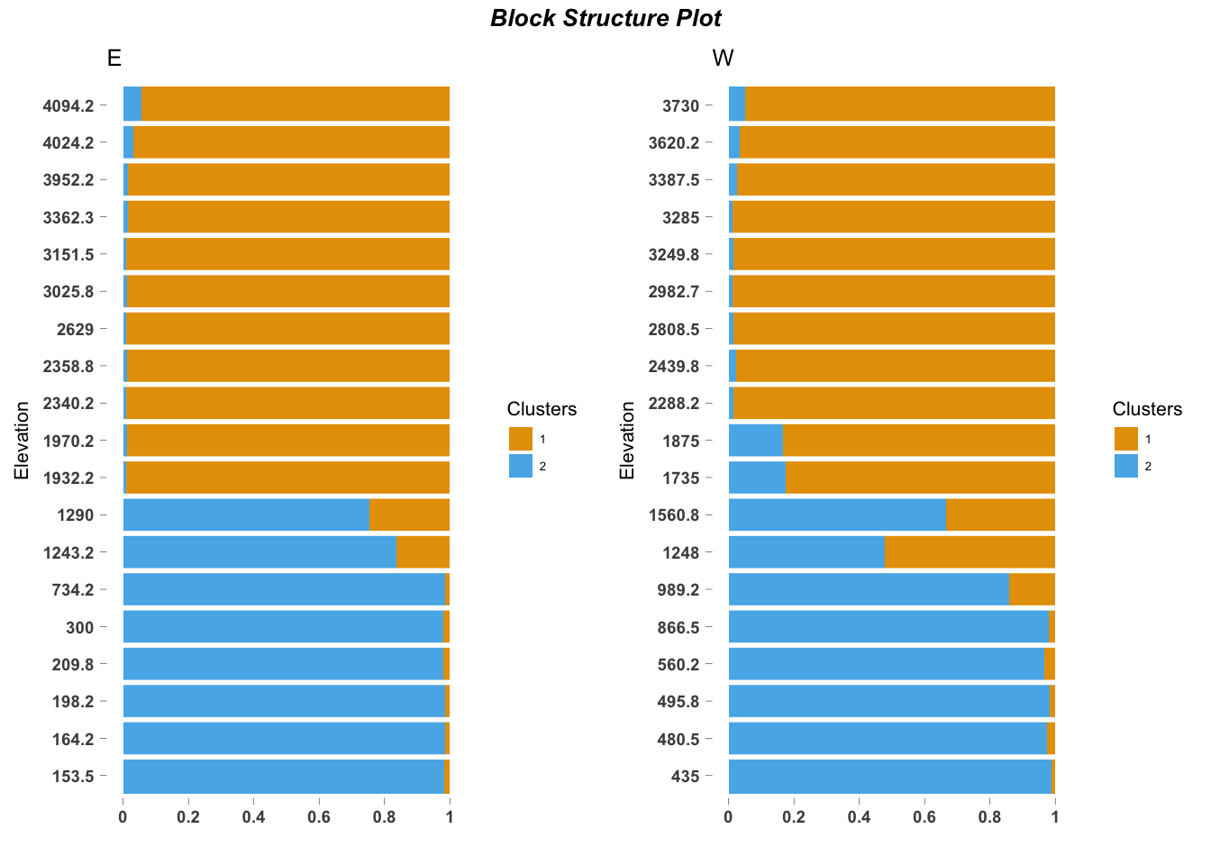
topics$L## [1] -2557.674sessionInfo()## R version 3.4.2 (2017-09-28)
## Platform: x86_64-apple-darwin15.6.0 (64-bit)
## Running under: macOS Sierra 10.12.6
##
## Matrix products: default
## BLAS: /Library/Frameworks/R.framework/Versions/3.4/Resources/lib/libRblas.0.dylib
## LAPACK: /Library/Frameworks/R.framework/Versions/3.4/Resources/lib/libRlapack.dylib
##
## locale:
## [1] en_US.UTF-8/en_US.UTF-8/en_US.UTF-8/C/en_US.UTF-8/en_US.UTF-8
##
## attached base packages:
## [1] parallel grid stats graphics grDevices utils datasets
## [8] methods base
##
## other attached packages:
## [1] slam_0.1-40 methClust_0.1.0 ecostructure_0.99.1
## [4] Biobase_2.38.0 BiocGenerics_0.24.0 maptools_0.9-2
## [7] SpatialExtremes_2.0-5 phytools_0.6-20 maps_3.2.0
## [10] ape_5.0 gridExtra_2.3 rgdal_1.2-15
## [13] raster_2.5-8 sp_1.2-5 maptpx_1.9-3
## [16] CountClust_1.5.1 ggplot2_2.2.1
##
## loaded via a namespace (and not attached):
## [1] viridisLite_0.2.0 splines_3.4.2
## [3] gtools_3.5.0 expm_0.999-2
## [5] stats4_3.4.2 latticeExtra_0.6-28
## [7] animation_2.5 yaml_2.1.14
## [9] numDeriv_2016.8-1 backports_1.1.0
## [11] lattice_0.20-35 limma_3.34.1
## [13] quadprog_1.5-5 phangorn_2.3.1
## [15] digest_0.6.12 RColorBrewer_1.1-2
## [17] colorspace_1.3-2 picante_1.6-2
## [19] cowplot_0.9.1 htmltools_0.3.6
## [21] Matrix_1.2-12 plyr_1.8.4
## [23] pkgconfig_2.0.1 mvtnorm_1.0-6
## [25] scales_0.5.0 tibble_1.3.4
## [27] combinat_0.0-8 mgcv_1.8-20
## [29] hexbin_1.27.1 nnet_7.3-12
## [31] lazyeval_0.2.1 rasterVis_0.41
## [33] mnormt_1.5-5 survival_2.41-3
## [35] magrittr_1.5 evaluate_0.10.1
## [37] msm_1.6.4 nlme_3.1-131
## [39] MASS_7.3-47 foreign_0.8-69
## [41] vegan_2.4-4 tools_3.4.2
## [43] stringr_1.2.0 munsell_0.4.3
## [45] cluster_2.0.6 plotrix_3.6-6
## [47] compiler_3.4.2 clusterGeneration_1.3.4
## [49] rlang_0.1.4 igraph_1.1.2
## [51] rmarkdown_1.8 boot_1.3-20
## [53] gtable_0.2.0 flexmix_2.3-14
## [55] reshape2_1.4.2 zoo_1.8-0
## [57] knitr_1.17 fastmatch_1.1-0
## [59] rprojroot_1.2 permute_0.9-4
## [61] modeltools_0.2-21 stringi_1.1.5
## [63] SQUAREM_2017.10-1 Rcpp_0.12.13
## [65] scatterplot3d_0.3-40 coda_0.19-1This R Markdown site was created with workflowr