Creating assemblage fields from cells by birds presence absences
Kushal K Dey
12/17/2017
library(ggplot2)
library(ggthemes)
library(maps)
Constructed Assemblage
new_assemblage <- get(load("../output/constructed_assemblage.rda"))Original Assemblage
old_assemblage <- readRDS("../data/global_disp_field_matrix_breeding_birds_rds.rds")Assemblage Map Function
We load the latitude and longitude data for each site for the newly constructed assemblage as well as the older assemblage.
latlong <- get(load("../data/LatLongCells_frame.rda"))We write the plotting function.
world_map <- map_data("world")
world_map <- world_map[world_map$region != "Antarctica",] # intercourse antarctica

p <- ggplot() + coord_fixed() +
  xlab("") + ylab("")

#Add map to base plot
base_world_messy <- p + geom_map(data=world_map, map = world_map, aes(group=group, map_id=region), colour="white", fill="white", size=0.05, alpha=1/4)

cleanup <-
  theme(panel.grid.major = element_blank(), panel.grid.minor = element_blank(),
        panel.background = element_rect(fill = 'white', colour = 'white'),
        axis.line = element_line(colour = "white"), legend.position="none",
        axis.ticks=element_blank(), axis.text.x=element_blank(),
        axis.text.y=element_blank())

base_world <- base_world_messy + cleanup
PlotAssemblageIdx <- function(idx){
dat <- cbind.data.frame(latlong, new_assemblage[,idx])
colnames(dat) <- c("Latitude", "Longitude", "Value")
map_data_coloured <-
base_world +
geom_point(data=dat,
aes(x=Latitude, y=Longitude, colour=Value), size=0.5) +
scale_colour_gradient(low = "white", high = "black")
map_data_coloured
}Example Plots of sites
par(mfrow = c(10, 2))
PlotAssemblageIdx(500)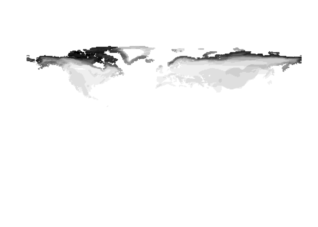
PlotAssemblageIdx(1000)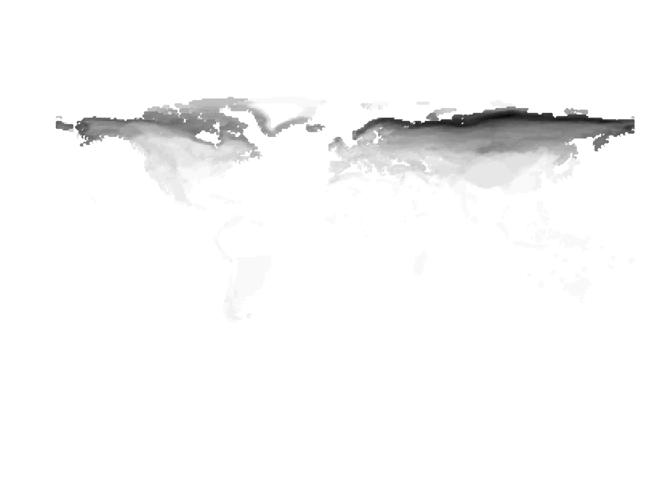
PlotAssemblageIdx(1500)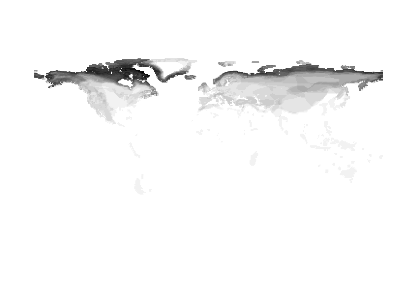
PlotAssemblageIdx(2000)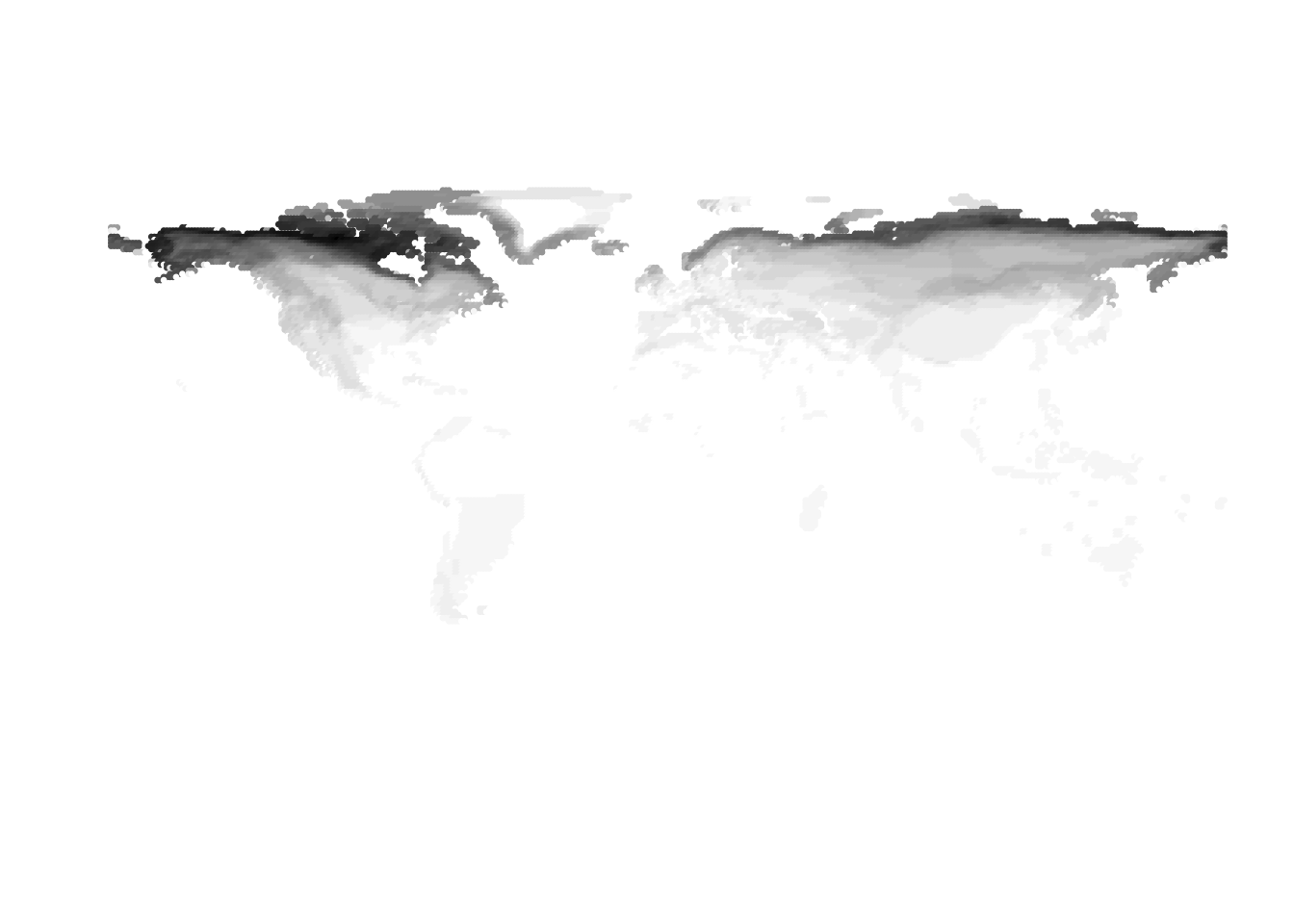
PlotAssemblageIdx(3000)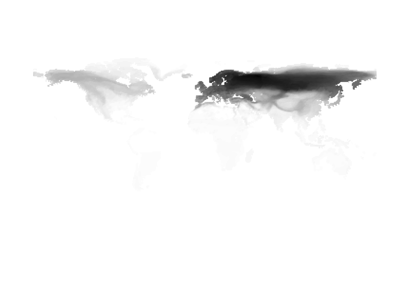
PlotAssemblageIdx(4000)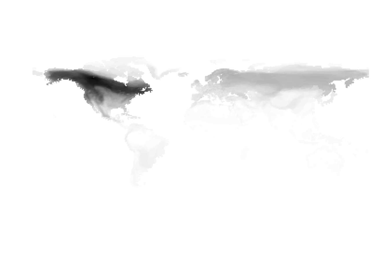
PlotAssemblageIdx(5000)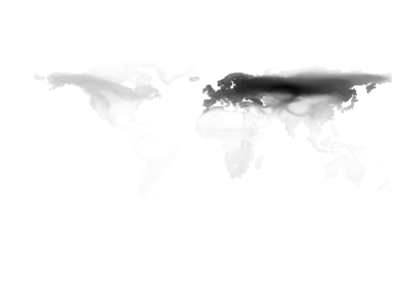
PlotAssemblageIdx(7000)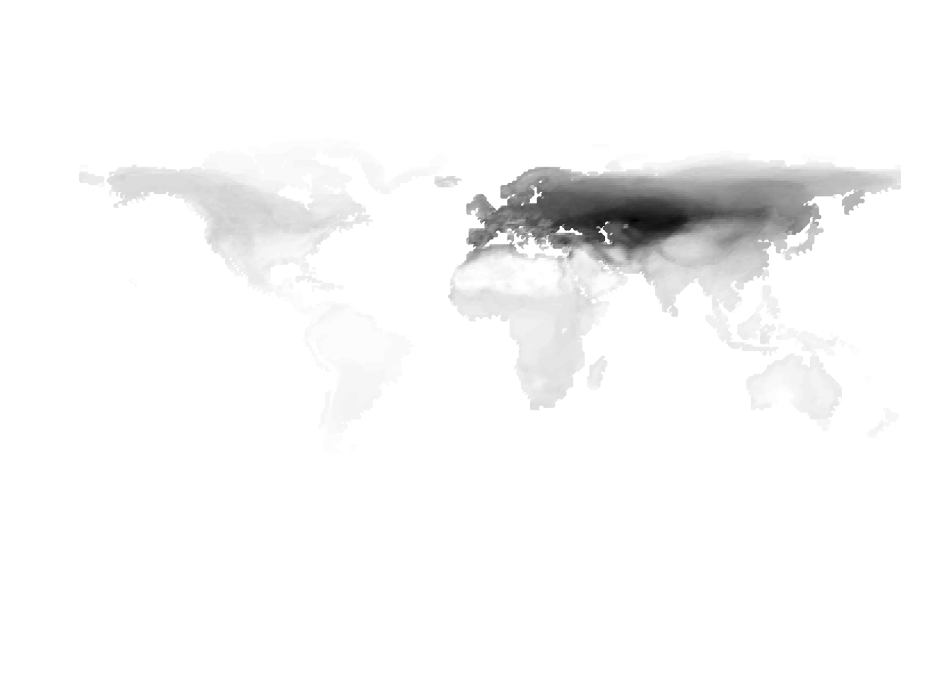
PlotAssemblageIdx(8000)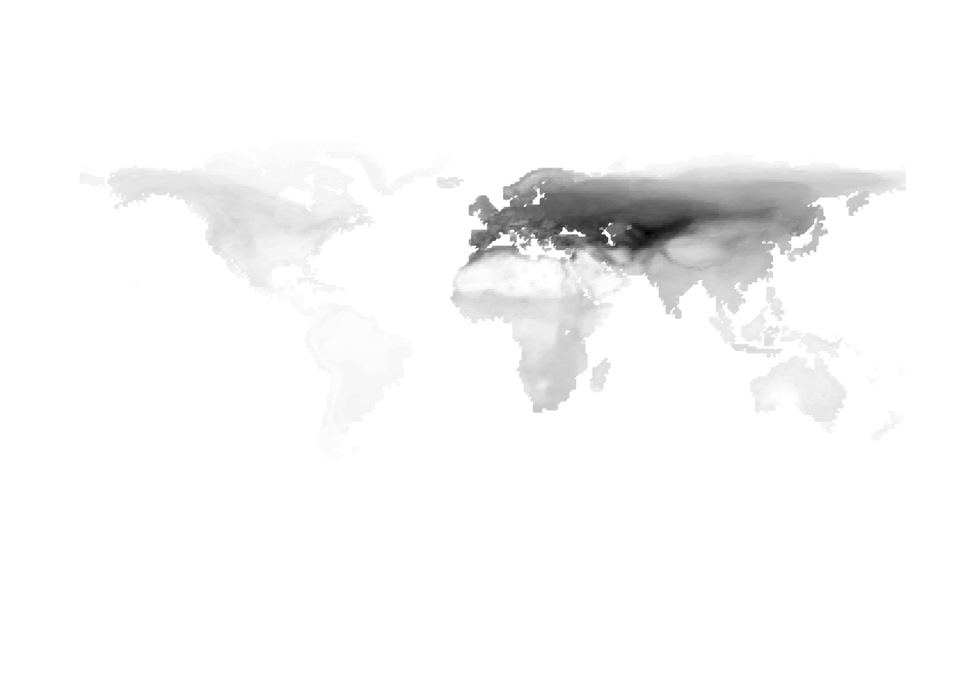
PlotAssemblageIdx(9000)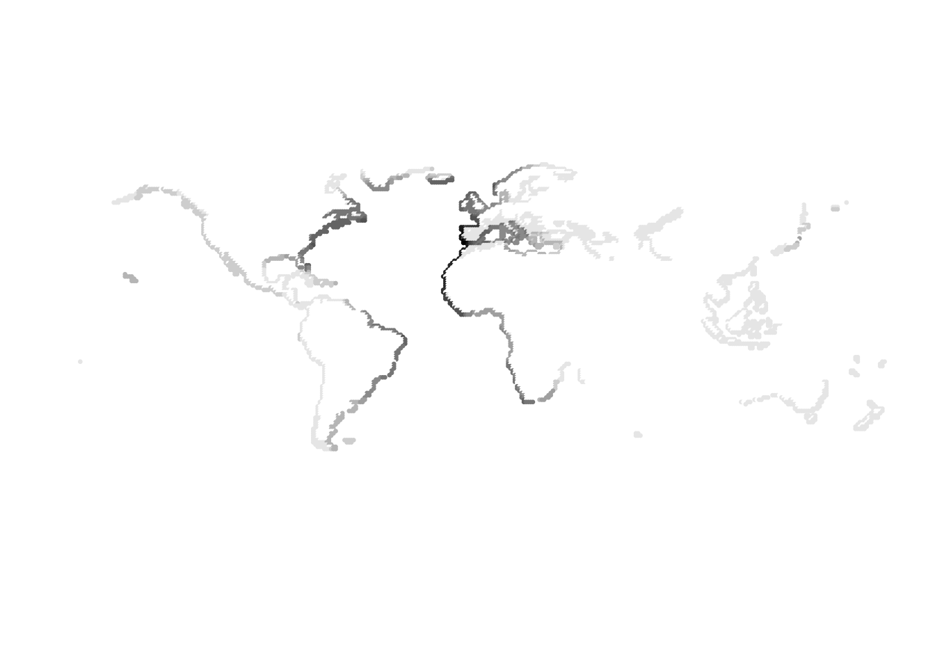
PlotAssemblageIdx(10000)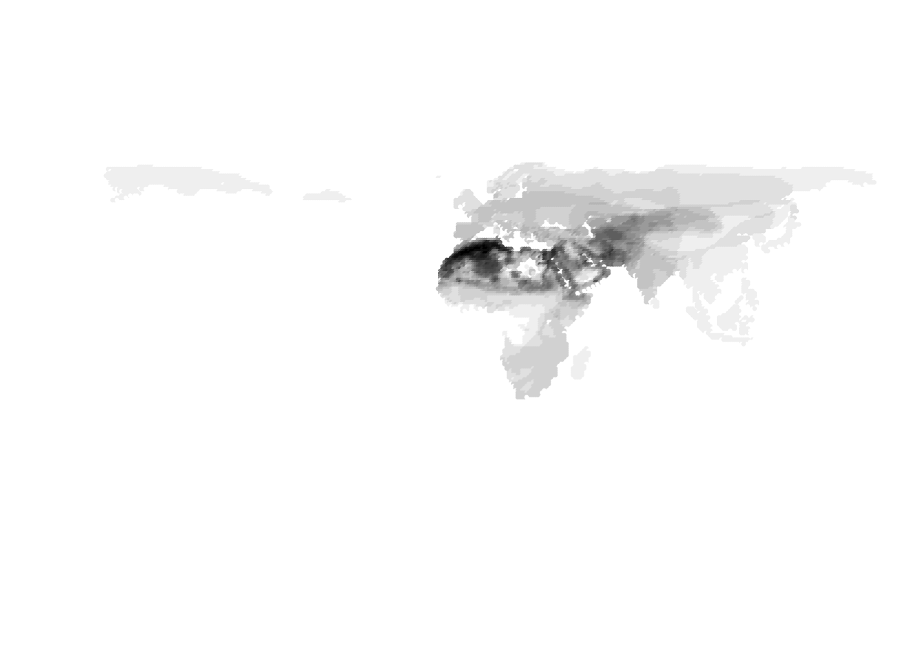
PlotAssemblageIdx(11000)
PlotAssemblageIdx(12000)
PlotAssemblageIdx(13000)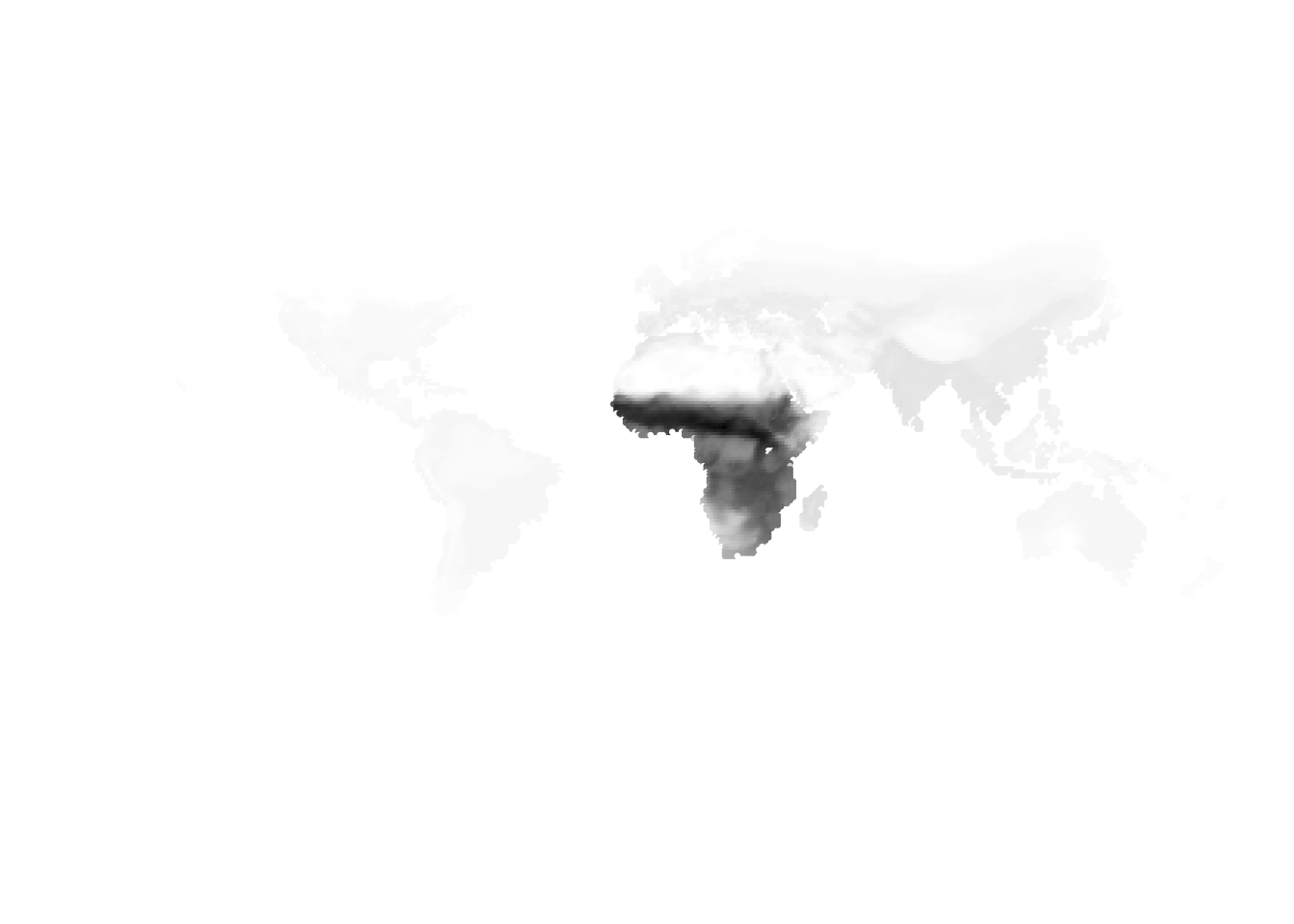
PlotAssemblageIdx(14000)
PlotAssemblageIdx(15000)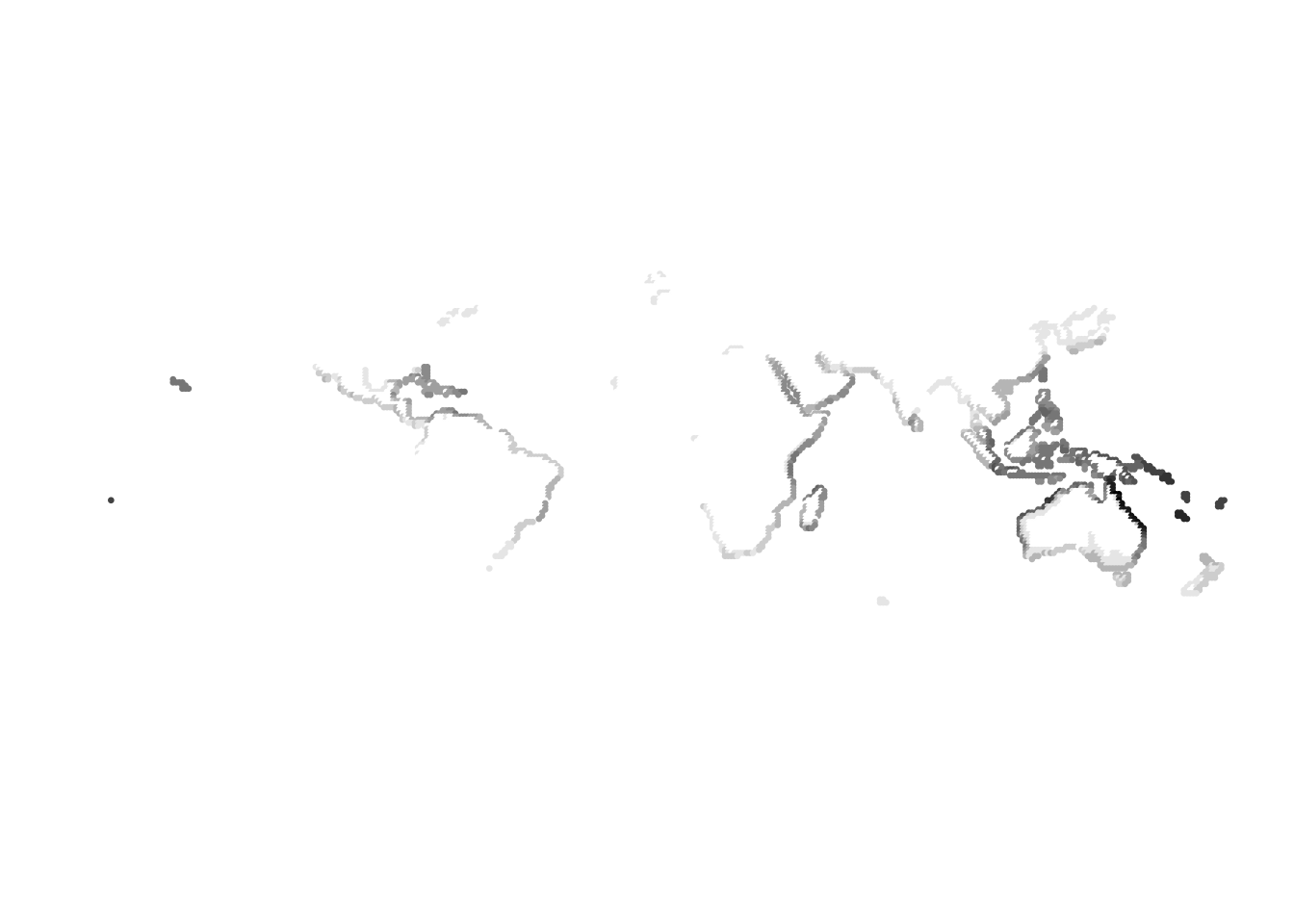
PlotAssemblageIdx(15500)
PlotAssemblageIdx(16000)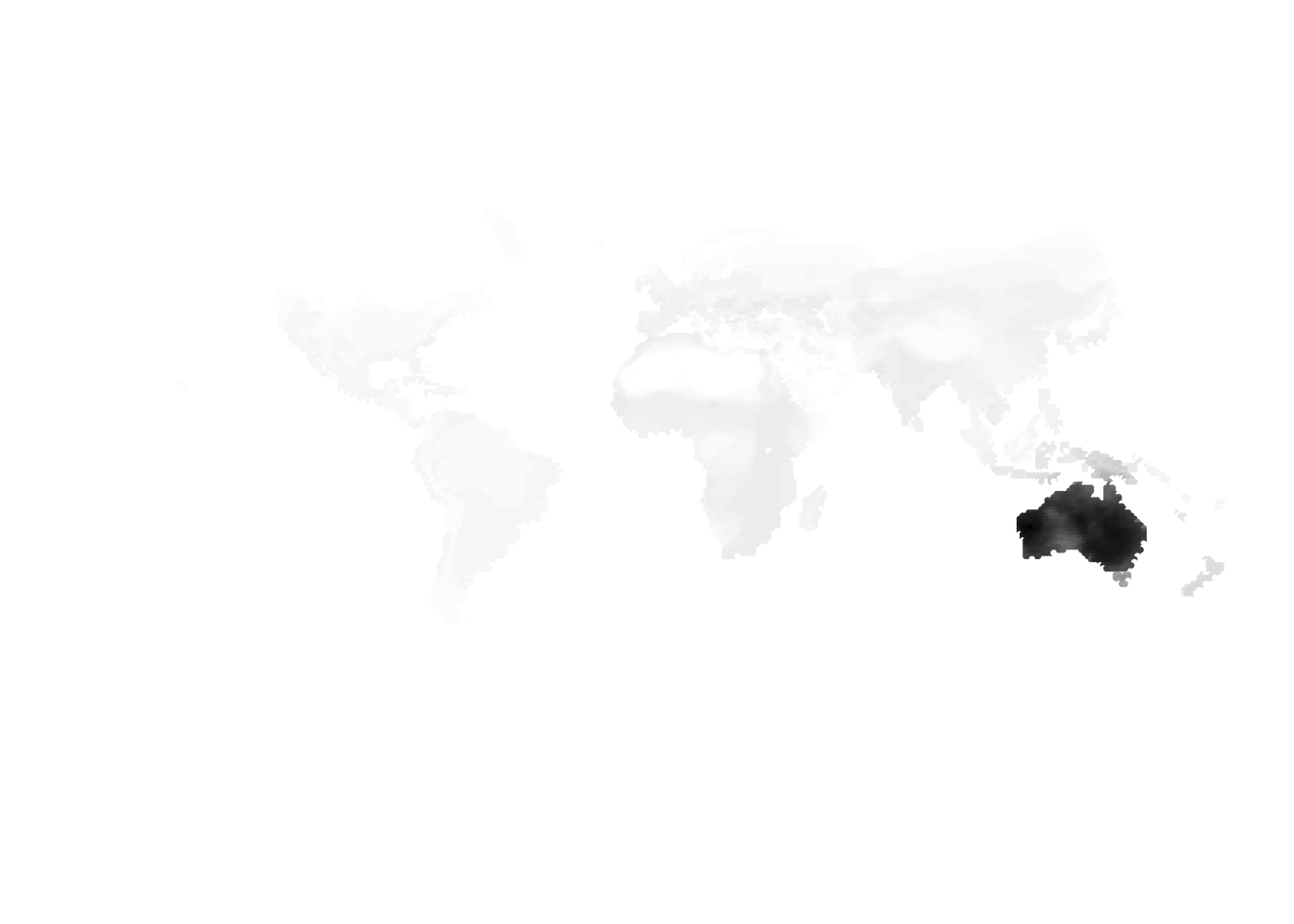
PlotAssemblageIdx(16500)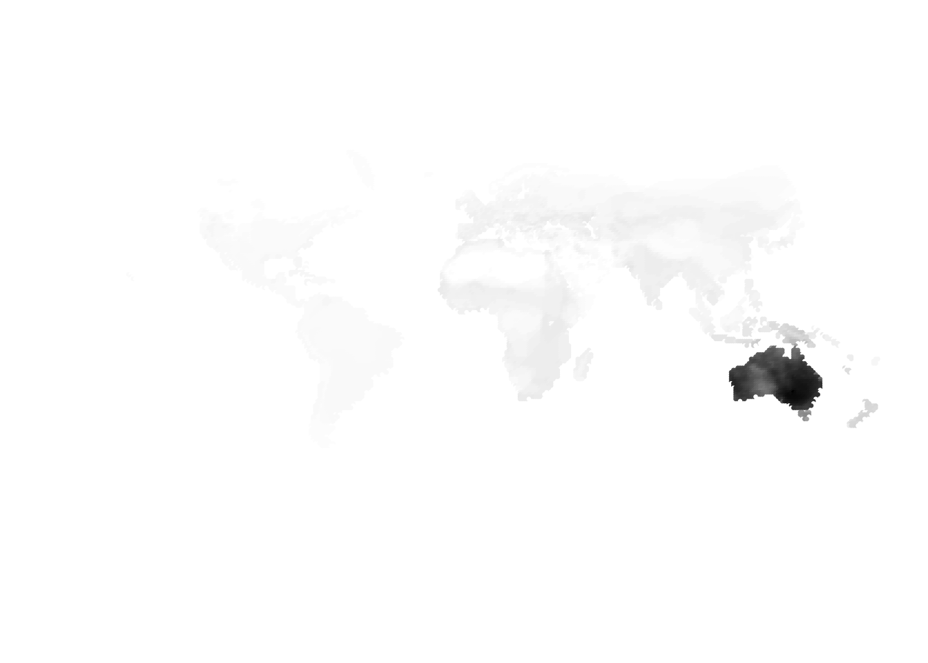
PlotAssemblageIdx(17000)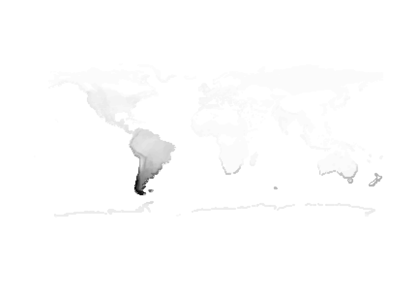
This R Markdown site was created with workflowr