Clines vs Clusters : Himalayan Birds abundance

We try to interpret if we are seeing continuous clines or dicrete clusters in the Himalayan birds abundance data.

library(ecostructure)
library(Biobase)

Load Data

data("himalayan_birds")
species_abundance_counts <- t(exprs(himalayan_birds));
site_metadata <- pData(himalayan_birds)
elevation_metadata=site_metadata$Elevation;
east_west_dir = site_metadata$WorE;

Ecos Fit

set.seed(1000)
fit <- ecos_fit(species_abundance_counts, K = 2, tol = 0.1, num_trials = 10)

## Fitting a Grade of Membership model
##             (Taddy M., AISTATS 2012, JMLR 22,
##             http://proceedings.mlr.press/v22/taddy12/taddy12.pdf)

## 
## Estimating on a 38 samples collection.
## Fit and Bayes Factor Estimation for K = 2
## log posterior increase: 18315.4, 83.3, 88.4, 0.6, done.
## log BF( 2 ) = 2175.01

## Fitting a Grade of Membership model
##             (Taddy M., AISTATS 2012, JMLR 22,
##             http://proceedings.mlr.press/v22/taddy12/taddy12.pdf)

## 
## Estimating on a 38 samples collection.
## Fit and Bayes Factor Estimation for K = 2
## log posterior increase: 2937.3, 10.8, 0.5, done.
## log BF( 2 ) = 1772.92

## Fitting a Grade of Membership model
##             (Taddy M., AISTATS 2012, JMLR 22,
##             http://proceedings.mlr.press/v22/taddy12/taddy12.pdf)

## 
## Estimating on a 38 samples collection.
## Fit and Bayes Factor Estimation for K = 2
## log posterior increase: 20698.2, 63.5, 12.4, 13.4, 6.6, 0.6, done.
## log BF( 2 ) = 1791.65

## Fitting a Grade of Membership model
##             (Taddy M., AISTATS 2012, JMLR 22,
##             http://proceedings.mlr.press/v22/taddy12/taddy12.pdf)

## 
## Estimating on a 38 samples collection.
## Fit and Bayes Factor Estimation for K = 2
## log posterior increase: 15913.2, 73.6, 0.7, done.
## log BF( 2 ) = 1922.38

## Fitting a Grade of Membership model
##             (Taddy M., AISTATS 2012, JMLR 22,
##             http://proceedings.mlr.press/v22/taddy12/taddy12.pdf)

## 
## Estimating on a 38 samples collection.
## Fit and Bayes Factor Estimation for K = 2
## log posterior increase: 2131.8, 61.4, 2, done.
## log BF( 2 ) = 1951.69

## Fitting a Grade of Membership model
##             (Taddy M., AISTATS 2012, JMLR 22,
##             http://proceedings.mlr.press/v22/taddy12/taddy12.pdf)

## 
## Estimating on a 38 samples collection.
## Fit and Bayes Factor Estimation for K = 2
## log posterior increase: 3565.7, 4, done.
## log BF( 2 ) = 1874.04

## Fitting a Grade of Membership model
##             (Taddy M., AISTATS 2012, JMLR 22,
##             http://proceedings.mlr.press/v22/taddy12/taddy12.pdf)

## 
## Estimating on a 38 samples collection.
## Fit and Bayes Factor Estimation for K = 2
## log posterior increase: 14118, 120, 45.1, 0.5, 0.3, 0.1, done.
## log BF( 2 ) = 1953.93

## Fitting a Grade of Membership model
##             (Taddy M., AISTATS 2012, JMLR 22,
##             http://proceedings.mlr.press/v22/taddy12/taddy12.pdf)

## 
## Estimating on a 38 samples collection.
## Fit and Bayes Factor Estimation for K = 2
## log posterior increase: 2411.6, 47.5, 2.1, done.
## log BF( 2 ) = 1950.96

## Fitting a Grade of Membership model
##             (Taddy M., AISTATS 2012, JMLR 22,
##             http://proceedings.mlr.press/v22/taddy12/taddy12.pdf)

## 
## Estimating on a 38 samples collection.
## Fit and Bayes Factor Estimation for K = 2
## log posterior increase: 20280.2, 88.5, 14.4, 4.2, 14.1, done.
## log BF( 2 ) = 2186.57

## Fitting a Grade of Membership model
##             (Taddy M., AISTATS 2012, JMLR 22,
##             http://proceedings.mlr.press/v22/taddy12/taddy12.pdf)

## 
## Estimating on a 38 samples collection.
## Fit and Bayes Factor Estimation for K = 2
## log posterior increase: 23791.2, 31, 10.2, 25.1, 0.7, done.
## log BF( 2 ) = 1936.48

ecos_blocks(fit$omega,
            blocker_metadata = east_west_dir,
            order_metadata = elevation_metadata)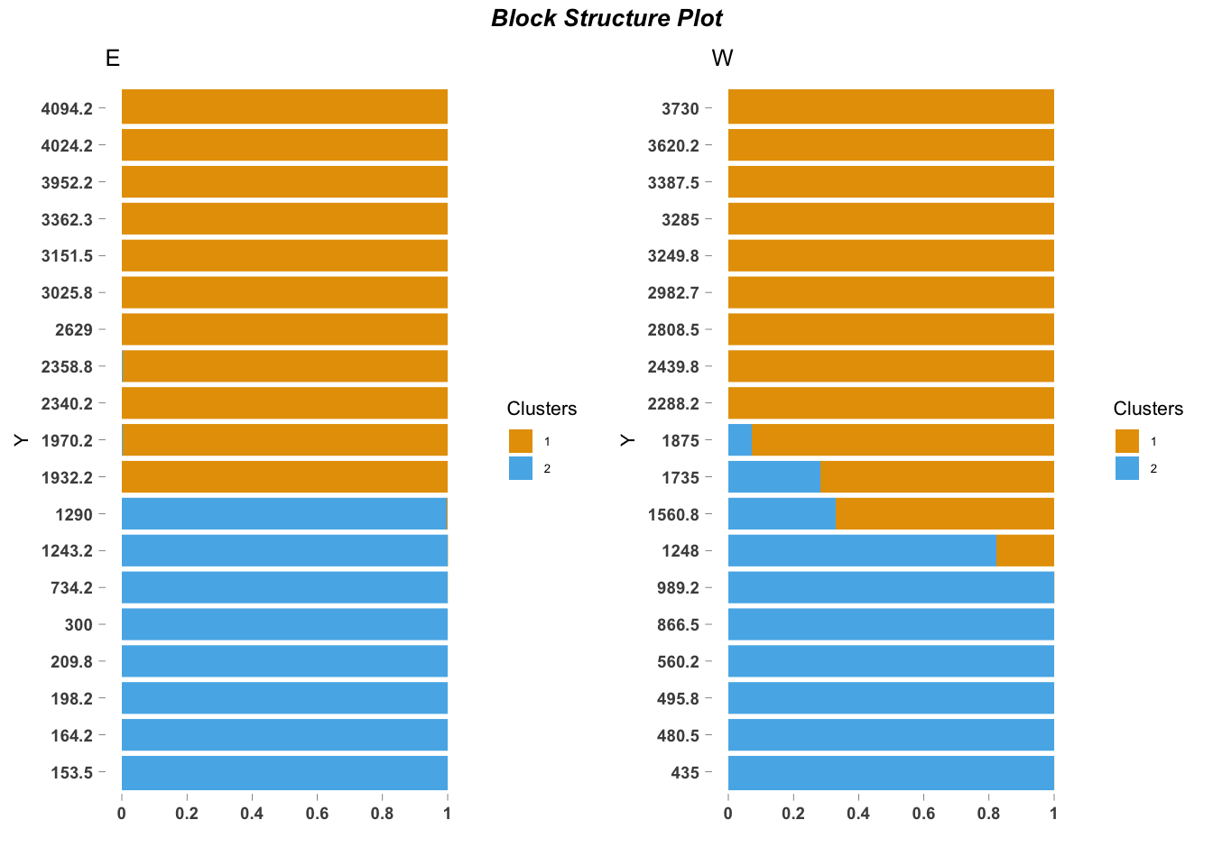

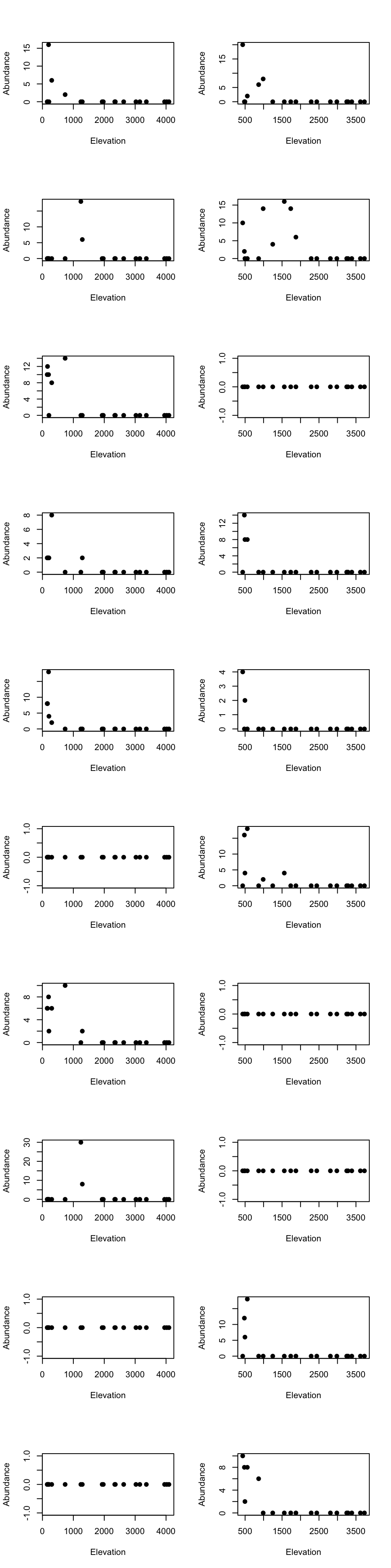
Differences between clusters

tmp1 <- fit$theta[order(fit$theta[,2] - fit$theta[,1], decreasing = TRUE)[1:10],]
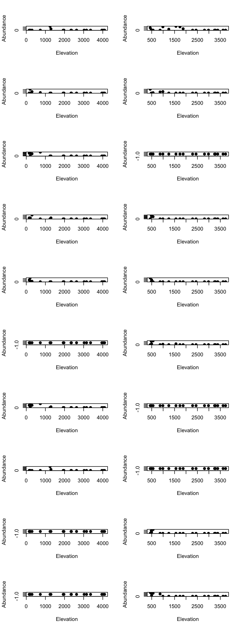
tmp2 <- fit$theta[order(fit$theta[,1] - fit$theta[,2], decreasing = TRUE)[1:10],]

Low elevational cluster species

par(mfrow=c(10, 2))

for(m in 1:10){
  tmp_dat <- species_abundance_counts[which(east_west_dir == "E"), rownames(tmp1)[m]]
  ele_dat <- elevation_metadata[which(east_west_dir == "E")]
  plot(ele_dat, tmp_dat, pch= 20, xlab = "Elevation", ylab = "Abundance", cex = 1.5)

  tmp_dat <- species_abundance_counts[which(east_west_dir == "W"), rownames(tmp1)[m]]
  ele_dat <- elevation_metadata[which(east_west_dir == "W")]
  plot(ele_dat, tmp_dat, pch= 20, xlab = "Elevation", ylab = "Abundance", cex = 1.5)
}

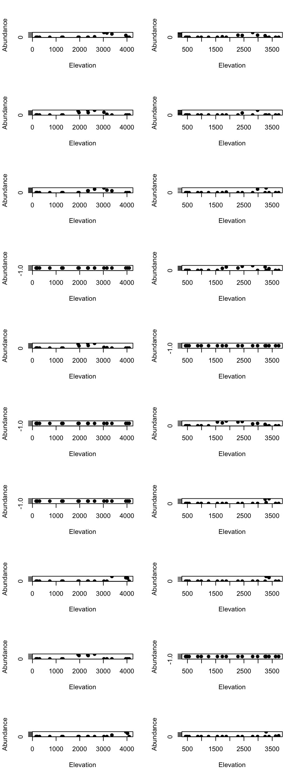
High elevational cluster species

par(mfrow=c(10, 2))

for(m in 1:10){
  tmp_dat <- species_abundance_counts[which(east_west_dir == "E"), rownames(tmp2)[m]]
  ele_dat <- elevation_metadata[which(east_west_dir == "E")]
  plot(ele_dat, tmp_dat, pch= 20, xlab = "Elevation", ylab = "Abundance", cex = 1.5)

  tmp_dat <- species_abundance_counts[which(east_west_dir == "W"), rownames(tmp2)[m]]
  ele_dat <- elevation_metadata[which(east_west_dir == "W")]
  plot(ele_dat, tmp_dat, pch= 20, xlab = "Elevation", ylab = "Abundance", cex = 1.5)
}

Ecos Fit

set.seed(1000)
fit2 <- ecos_fit(species_abundance_counts, K = 3, tol = 0.1, num_trials = 10)

## Fitting a Grade of Membership model
##             (Taddy M., AISTATS 2012, JMLR 22,
##             http://proceedings.mlr.press/v22/taddy12/taddy12.pdf)

## 
## Estimating on a 38 samples collection.
## Fit and Bayes Factor Estimation for K = 3
## log posterior increase: 2592.7, 54.1, 36.6, 1.4, 6.2, done.
## log BF( 3 ) = 2569.15

## Fitting a Grade of Membership model
##             (Taddy M., AISTATS 2012, JMLR 22,
##             http://proceedings.mlr.press/v22/taddy12/taddy12.pdf)

## 
## Estimating on a 38 samples collection.
## Fit and Bayes Factor Estimation for K = 3
## log posterior increase: 3346.6, 61.5, 26.2, 3.9, 12.6, done.
## log BF( 3 ) = 2578.68

## Fitting a Grade of Membership model
##             (Taddy M., AISTATS 2012, JMLR 22,
##             http://proceedings.mlr.press/v22/taddy12/taddy12.pdf)

## 
## Estimating on a 38 samples collection.
## Fit and Bayes Factor Estimation for K = 3
## log posterior increase: 3501, 74.4, 101, 8.4, 3.7, 9.8, 42.1, 4.5, 0.4, done.
## log BF( 3 ) = 2531.7

## Fitting a Grade of Membership model
##             (Taddy M., AISTATS 2012, JMLR 22,
##             http://proceedings.mlr.press/v22/taddy12/taddy12.pdf)

## 
## Estimating on a 38 samples collection.
## Fit and Bayes Factor Estimation for K = 3
## log posterior increase: 2788.2, 110.6, 49.6, 30.7, 5.9, 1, 0, done.
## log BF( 3 ) = 2528.31

## Fitting a Grade of Membership model
##             (Taddy M., AISTATS 2012, JMLR 22,
##             http://proceedings.mlr.press/v22/taddy12/taddy12.pdf)

## 
## Estimating on a 38 samples collection.
## Fit and Bayes Factor Estimation for K = 3
## log posterior increase: 3031.2, 22.3, 20, 17.7, done.
## log BF( 3 ) = 2432.48

## Fitting a Grade of Membership model
##             (Taddy M., AISTATS 2012, JMLR 22,
##             http://proceedings.mlr.press/v22/taddy12/taddy12.pdf)

## 
## Estimating on a 38 samples collection.
## Fit and Bayes Factor Estimation for K = 3
## log posterior increase: 4046.2, 5.7, 1.7, done.
## log BF( 3 ) = 2532.88

## Fitting a Grade of Membership model
##             (Taddy M., AISTATS 2012, JMLR 22,
##             http://proceedings.mlr.press/v22/taddy12/taddy12.pdf)

## 
## Estimating on a 38 samples collection.
## Fit and Bayes Factor Estimation for K = 3
## log posterior increase: 2596.6, 26.5, 7.1, 10.3, 51.2, 16.3, 10.8, 1.3, done.
## log BF( 3 ) = 2568.82

## Fitting a Grade of Membership model
##             (Taddy M., AISTATS 2012, JMLR 22,
##             http://proceedings.mlr.press/v22/taddy12/taddy12.pdf)

## 
## Estimating on a 38 samples collection.
## Fit and Bayes Factor Estimation for K = 3
## log posterior increase: 2956.1, 134.4, 11.1, 1, done.
## log BF( 3 ) = 2437.03

## Fitting a Grade of Membership model
##             (Taddy M., AISTATS 2012, JMLR 22,
##             http://proceedings.mlr.press/v22/taddy12/taddy12.pdf)

## 
## Estimating on a 38 samples collection.
## Fit and Bayes Factor Estimation for K = 3
## log posterior increase: 3281.8, 92.1, 37.7, 40.8, 0.7, 0.1, done.
## log BF( 3 ) = 2220.24

## Fitting a Grade of Membership model
##             (Taddy M., AISTATS 2012, JMLR 22,
##             http://proceedings.mlr.press/v22/taddy12/taddy12.pdf)

## 
## Estimating on a 38 samples collection.
## Fit and Bayes Factor Estimation for K = 3
## log posterior increase: 18024.6, 24.7, 7.7, 11.2, 8.5, 28.1, 21.3, 0.8, done.
## log BF( 3 ) = 2536.49

ecos_blocks(fit$omega,
            blocker_metadata = east_west_dir,
            order_metadata = elevation_metadata)

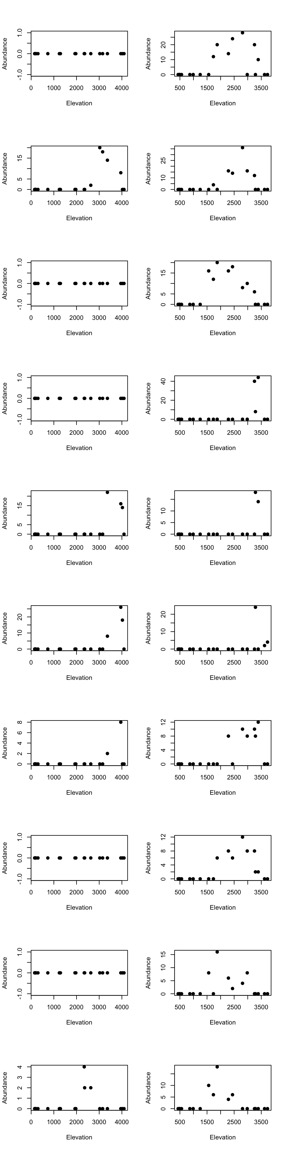
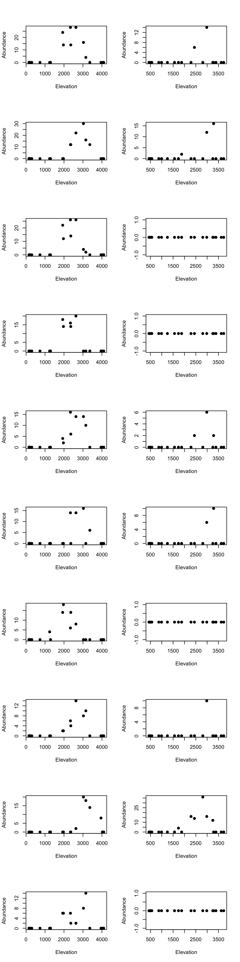
High elevational cluster species

par(mfrow=c(10, 2))

for(m in 1:10){
  tmp_dat <- species_abundance_counts[which(east_west_dir == "E"), rownames(fit2$theta[order(fit2$theta[,1], decreasing = TRUE)[1:10],])[m]]
  ele_dat <- elevation_metadata[which(east_west_dir == "E")]
  plot(ele_dat, tmp_dat, pch= 20, xlab = "Elevation", ylab = "Abundance", cex = 1.5)

  tmp_dat <- species_abundance_counts[which(east_west_dir == "W"), rownames(fit2$theta[order(fit2$theta[,1], decreasing = TRUE)[1:10],])[m]]
  ele_dat <- elevation_metadata[which(east_west_dir == "W")]
  plot(ele_dat, tmp_dat, pch= 20, xlab = "Elevation", ylab = "Abundance", cex = 1.5)
}

Low elevational cluster species

par(mfrow=c(10, 2))

for(m in 1:10){
  tmp_dat <- species_abundance_counts[which(east_west_dir == "E"), rownames(fit2$theta[order(fit2$theta[,2], decreasing = TRUE)[1:10],])[m]]
  ele_dat <- elevation_metadata[which(east_west_dir == "E")]
  plot(ele_dat, tmp_dat, pch= 20, xlab = "Elevation", ylab = "Abundance", cex = 1.5)

  tmp_dat <- species_abundance_counts[which(east_west_dir == "W"), rownames(fit2$theta[order(fit2$theta[,2], decreasing = TRUE)[1:10],])[m]]
  ele_dat <- elevation_metadata[which(east_west_dir == "W")]
  plot(ele_dat, tmp_dat, pch= 20, xlab = "Elevation", ylab = "Abundance", cex = 1.5)
}

Medium elevational cluster species

par(mfrow=c(10, 2))

for(m in 1:10){
  tmp_dat <- species_abundance_counts[which(east_west_dir == "E"), rownames(fit2$theta[order(fit2$theta[,3], decreasing = TRUE)[1:10],])[m]]
  ele_dat <- elevation_metadata[which(east_west_dir == "E")]
  plot(ele_dat, tmp_dat, pch= 20, xlab = "Elevation", ylab = "Abundance", cex = 1.5)

  tmp_dat <- species_abundance_counts[which(east_west_dir == "W"), rownames(fit2$theta[order(fit2$theta[,3], decreasing = TRUE)[1:10],])[m]]
  ele_dat <- elevation_metadata[which(east_west_dir == "W")]
  plot(ele_dat, tmp_dat, pch= 20, xlab = "Elevation", ylab = "Abundance", cex = 1.5)
}

This R Markdown site was created with workflowr

Clines vs Clusters : Himalayan Birds abundance

Kushal K Dey

8/24/2018

Load Data

Ecos Fit

Differences between clusters

Low elevational cluster species

High elevational cluster species

Ecos Fit

High elevational cluster species

Low elevational cluster species

Medium elevational cluster species