GTEx rank issue and imputation problem
Kushal K. Dey and Rahul Mazumder
11/25/2019
Last updated: 2020-03-08
workflowr checks: (Click a bullet for more information)-
✖ R Markdown file: uncommitted changes
The R Markdown is untracked by Git. To know which version of the R Markdown file created these results, you’ll want to first commit it to the Git repo. If you’re still working on the analysis, you can ignore this warning. When you’re finished, you can runwflow_publishto commit the R Markdown file and build the HTML. -
✔ Environment: empty
Great job! The global environment was empty. Objects defined in the global environment can affect the analysis in your R Markdown file in unknown ways. For reproduciblity it’s best to always run the code in an empty environment.
-
✔ Seed:
set.seed(20190721)The command
set.seed(20190721)was run prior to running the code in the R Markdown file. Setting a seed ensures that any results that rely on randomness, e.g. subsampling or permutations, are reproducible. -
✔ Session information: recorded
Great job! Recording the operating system, R version, and package versions is critical for reproducibility.
-
Great! You are using Git for version control. Tracking code development and connecting the code version to the results is critical for reproducibility. The version displayed above was the version of the Git repository at the time these results were generated.✔ Repository version: 47185fd
Note that you need to be careful to ensure that all relevant files for the analysis have been committed to Git prior to generating the results (you can usewflow_publishorwflow_git_commit). workflowr only checks the R Markdown file, but you know if there are other scripts or data files that it depends on. Below is the status of the Git repository when the results were generated:
Note that any generated files, e.g. HTML, png, CSS, etc., are not included in this status report because it is ok for generated content to have uncommitted changes.Ignored files: Ignored: .DS_Store Ignored: .Rhistory Ignored: .Rproj.user/ Ignored: docs/.DS_Store Ignored: draft/ Ignored: output/output_sparse/ Untracked files: Untracked: .gitignore~ Untracked: analysis/band_prec_robocov.Rmd Untracked: analysis/blood_corspan_robospan_probospan.Rmd Untracked: analysis/corspan_robospan_probospan.Rmd Untracked: analysis/diff_robospan_examples.Rmd Untracked: analysis/eigenvalues_hub.Rmd Untracked: analysis/figure2.Rmd Untracked: analysis/gtex_analysis_robocov_examples.Rmd Untracked: analysis/gtex_pRobocov_pRobospan.Rmd Untracked: analysis/gtex_predictive_robocov.Rmd Untracked: analysis/gtex_rank_imputation.Rmd Untracked: analysis/gtex_robocov.Rmd Untracked: analysis/gtex_robocov_ex_robospan.Rmd Untracked: analysis/housekeeping_PPI_MR_enrichment.Rmd Untracked: analysis/hub_robocov.Rmd Untracked: analysis/mean_robocov.Rmd Untracked: analysis/pLI_shet_robospan_probospan.Rmd Untracked: analysis/predictive_analytics_gtex.Rmd Untracked: analysis/robocov_demo.Rmd Untracked: analysis/robospan_blood_compare.Rmd Untracked: analysis/robospan_corr.Rmd Untracked: analysis/summary_correlation_structure.Rmd Untracked: analysis/supp_figure_simulation.Rmd Untracked: analysis/toeplitz_robocov.Rmd Untracked: code/ robocov_sim.R Untracked: code/FDR_Robospan.R Untracked: code/Joints_Nov24.R Untracked: code/Untitled.R Untracked: code/annot_size.R Untracked: code/band_prec_ocor_sim.R Untracked: code/band_prec_pcor_sim.R Untracked: code/band_prec_sim.R Untracked: code/band_prec_sim2.R Untracked: code/bandprec_cor_sim.R Untracked: code/baseline_strategies.R Untracked: code/corr_span.R Untracked: code/correlation_gene_scores.R Untracked: code/gene_score_all_strategies.R Untracked: code/gtex_robocov.R Untracked: code/gtex_robocov_precision.R Untracked: code/hub_prec_cor_sim.R Untracked: code/hub_sim.R Untracked: code/hub_sim2.R Untracked: code/hub_sim_sparse.R Untracked: code/joint_robocov_model.R Untracked: code/joints_robocov.R Untracked: code/many_tau_star.R Untracked: code/maxHiCgene.R Untracked: code/meta_enrich.R Untracked: code/meta_single_enrich.R Untracked: code/postprocess_hub_toeplitz.R Untracked: code/predictive_analytics_hub.R Untracked: code/predictive_analytics_toeplitz.R Untracked: code/robocov_gtex.R Untracked: code/robocov_gtex_blood.R Untracked: code/robocov_gtex_brain.R Untracked: code/sim_results.R Untracked: code/single_tau_star.R Untracked: code/toeplitz_prec_cor_sim.R Untracked: code/toeplitz_sim.R Untracked: code/toeplitz_sim2.R Untracked: code/toeplitz_sim_sparse.R Untracked: data/Cor_pairwise_all_genes.rda Untracked: data/Gene_Scores/ Untracked: data/Robocov_Box_all_genes.rda Untracked: data/Robocov_Precision_all_genes.rda Untracked: data/gene_names_GTEX_V6.txt Untracked: data/housekeeping_genes.txt Untracked: data/person_tissue_genes_voom.rda Untracked: docs/figure/ Untracked: sim_code/ Unstaged changes: Modified: .gitignore Modified: analysis/index.Rmd
library(ggplot2)Warning: package 'ggplot2' was built under R version 3.5.2library(corrplot)corrplot 0.84 loadedlibrary(softImpute)Loading required package: MatrixLoaded softImpute 1.4In this script, we show that the GTEx tissue-wide gene expression data across individuals does not have a low rank factorization by looking at the eigen-values of the pairwise sample correlation matrix for a gene (PLIN1) from the GTEx genes.
We also show that imputation based models such as SoftImpute or simple median based interpolationwill fail miserably when the data contains extensive amounts of missing entries as in case of GTEx.
robocov_all_genes = get(load("/Users/kushaldey/Documents/Robocov-pages/data/Robocov_Box_all_genes.rda"))corrplot(robocov_all_genes[,,"ENSG00000186517"], diag = TRUE,
col = colorRampPalette(c("lightblue4", "lightblue2", "white", "indianred1", "indianred3"))(200),
tl.pos = "ld", tl.cex = 0.8, tl.col = "black",
rect.col = "white",na.label.col = "white",
method = "color", type = "lower", tl.srt=45)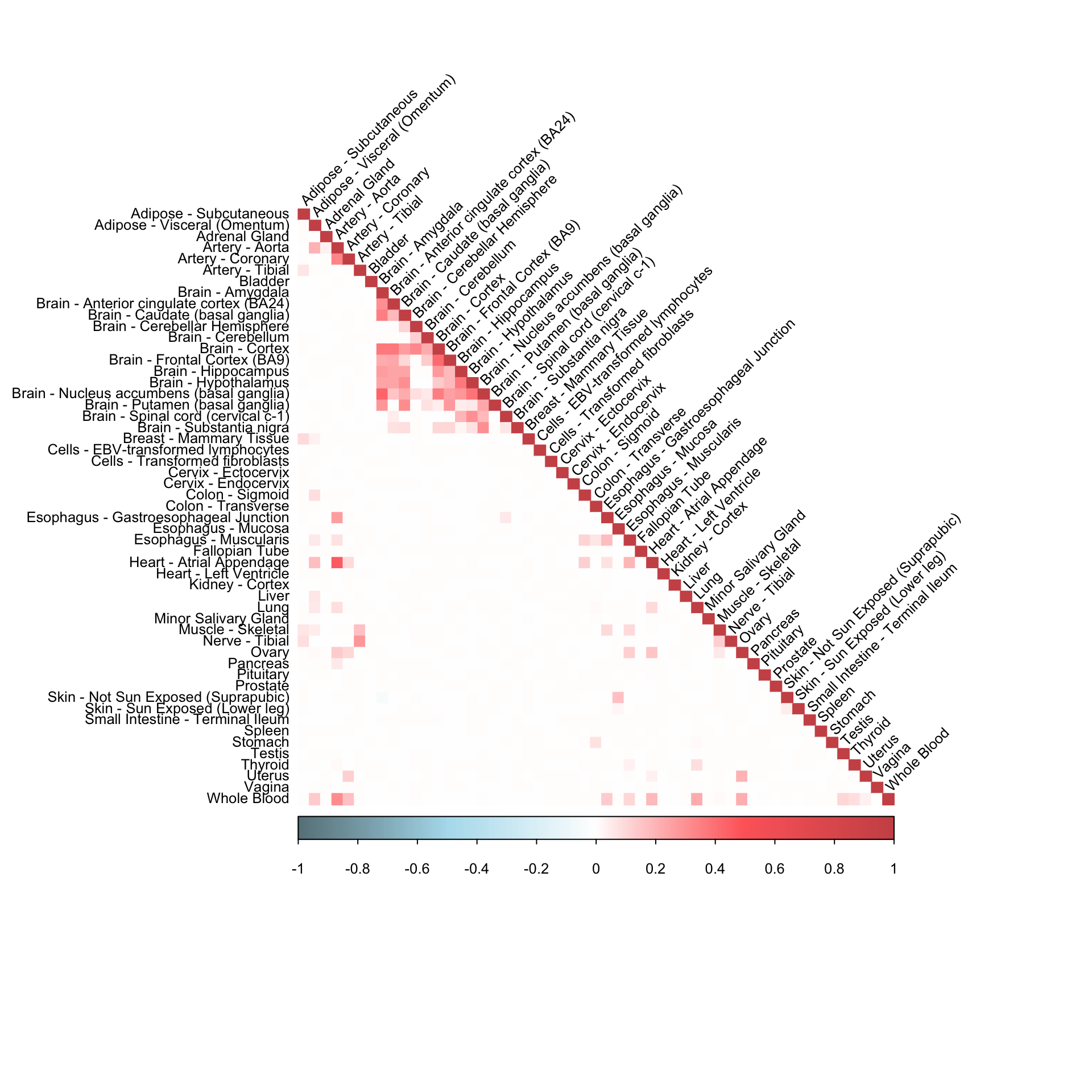
plot(eigen(as.matrix(robocov_all_genes[,,"ENSG00000186517"]))$values,
     xlab = "Features (tissues)", ylab = "Eigenvalues",
     main = "Eigenvalue trend for ARHGAP30 gene",
     col = "red",
     pch=20)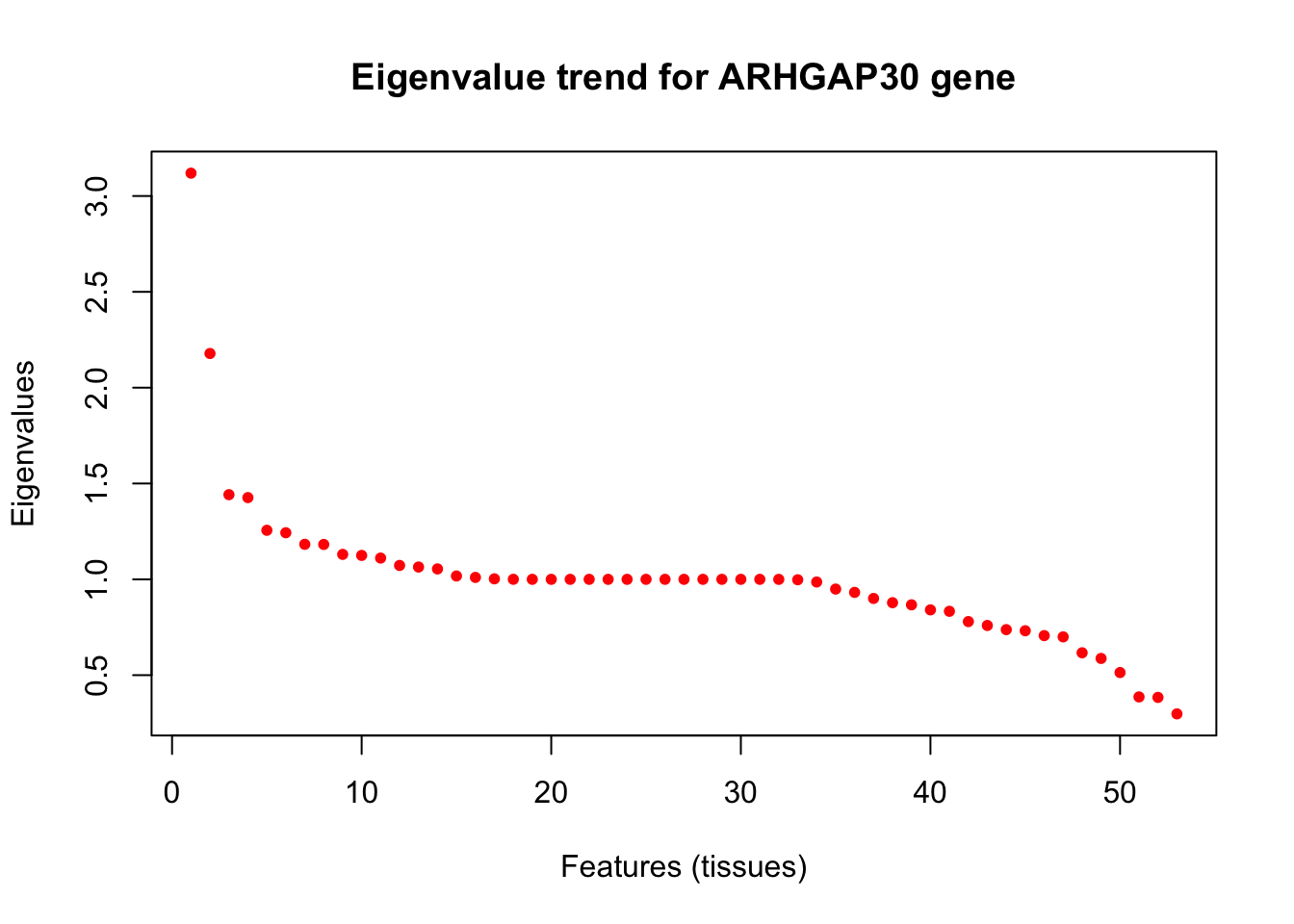
Column median imputation
dat = get(load("/Users/kushaldey/Documents/Robocov-pages/data/person_tissue_genes_voom.rda"))gene_dat = dat[,,"ENSG00000166819"]
gene_dat_imputed = apply(gene_dat, 2, function(x) {
y = x
y[which(is.na(x))] = median(x[!is.na(x)])
return(y)
})cormat = cor(gene_dat_imputed)
corrplot(cormat, diag = TRUE,
col = colorRampPalette(c("lightblue4", "lightblue2", "white", "indianred1", "indianred3"))(200),
tl.pos = "ld", tl.cex = 0.8, tl.col = "black",
rect.col = "white",na.label.col = "white",
method = "color", type = "lower", tl.srt=45)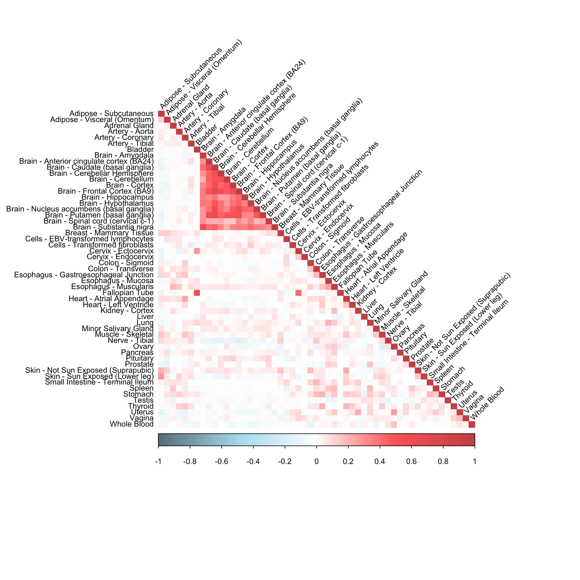
SoftImpute imputation
impute_method <- "svd"
matc=biScale(dat[,,"ENSG00000166819"],col.scale=TRUE,row.scale=FALSE,trace=TRUE)
Iter 1 Total Changes 855.6165
Iter 2 Total Changes 10.45967
Iter 3 Total Changes 0.3015997
Iter 4 Total Changes 0.02422897
Iter 5 Total Changes 0.004859336
Iter 6 Total Changes 0.001330174
Iter 7 Total Changes 0.0003840936
Iter 8 Total Changes 0.0001116573
Iter 9 Total Changes 3.246363e-05
Iter 10 Total Changes 9.43445e-06
Iter 11 Total Changes 2.741019e-06
Iter 12 Total Changes 7.962422e-07
Iter 13 Total Changes 2.312861e-07
Iter 14 Total Changes 6.718018e-08
Iter 15 Total Changes 1.951314e-08
Iter 16 Total Changes 5.667748e-09
Iter 17 Total Changes 1.646239e-09
Iter 18 Total Changes 4.781617e-10 fits3=softImpute(matc,rank.max=50,lambda=1,type=impute_method)
fitted_mat <- complete(dat[,,"ENSG00000166819"],fits3,unscale=T)
cormat <- cor(fitted_mat)corrplot(cormat, diag = TRUE,
col = colorRampPalette(c("lightblue4", "lightblue2", "white", "indianred1", "indianred3"))(200),
tl.pos = "ld", tl.cex = 0.8, tl.col = "black",
rect.col = "white",na.label.col = "white",
method = "color", type = "lower", tl.srt=45)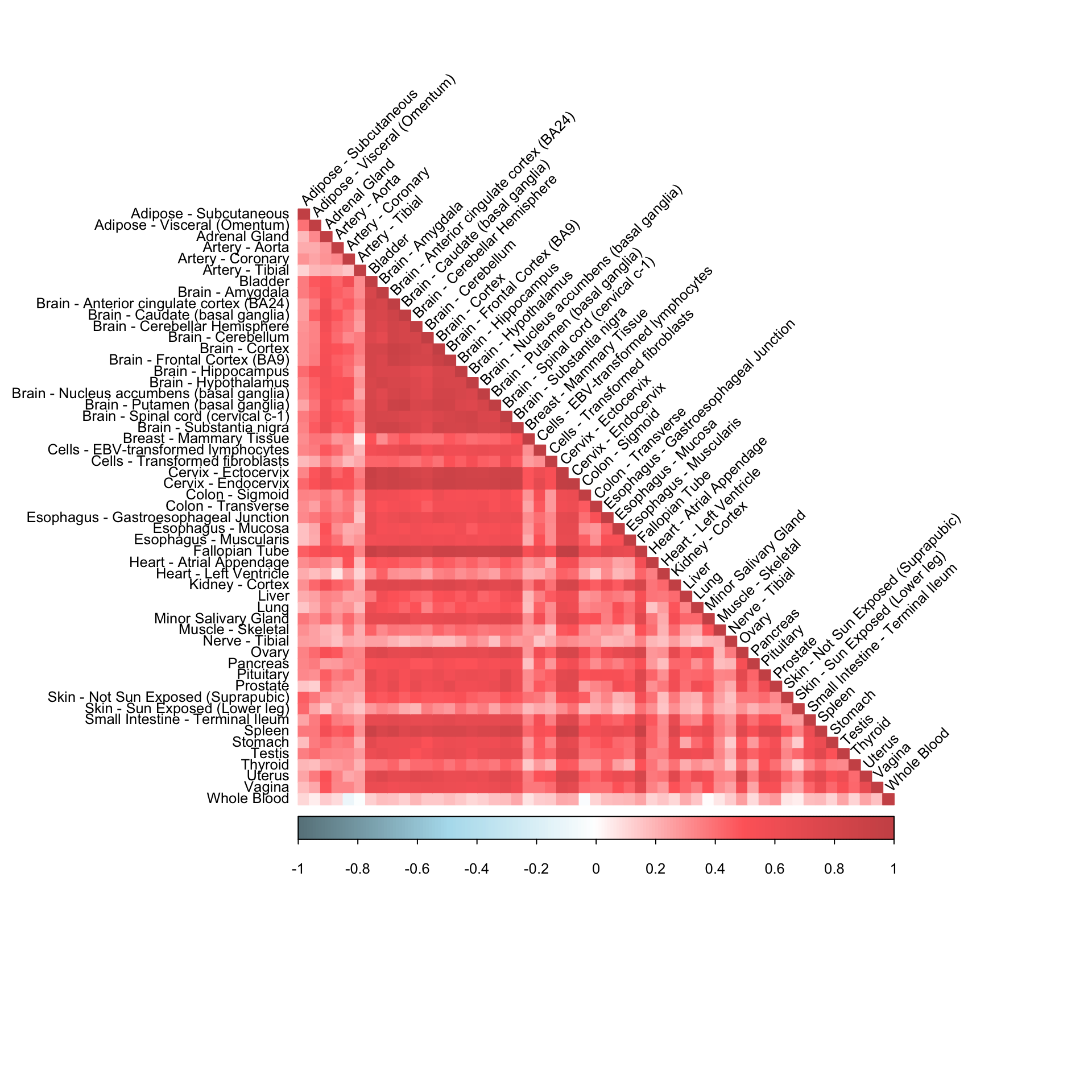
impute_method <- "svd"
matc=biScale(dat[,,"ENSG00000166819"],col.scale=TRUE,row.scale=FALSE,trace=TRUE)Iter 1 Total Changes 855.6165
Iter 2 Total Changes 10.45967
Iter 3 Total Changes 0.3015997
Iter 4 Total Changes 0.02422897
Iter 5 Total Changes 0.004859336
Iter 6 Total Changes 0.001330174
Iter 7 Total Changes 0.0003840936
Iter 8 Total Changes 0.0001116573
Iter 9 Total Changes 3.246363e-05
Iter 10 Total Changes 9.43445e-06
Iter 11 Total Changes 2.741019e-06
Iter 12 Total Changes 7.962422e-07
Iter 13 Total Changes 2.312861e-07
Iter 14 Total Changes 6.718018e-08
Iter 15 Total Changes 1.951314e-08
Iter 16 Total Changes 5.667748e-09
Iter 17 Total Changes 1.646239e-09
Iter 18 Total Changes 4.781617e-10 fits3=softImpute(matc,rank.max=50,lambda=1,type=impute_method)
fitted_mat <- complete(dat[,,"ENSG00000166819"],fits3,unscale=F)
cormat <- cor(fitted_mat)corrplot(cormat, diag = TRUE,
col = colorRampPalette(c("lightblue4", "lightblue2", "white", "indianred1", "indianred3"))(200),
tl.pos = "ld", tl.cex = 0.8, tl.col = "black",
rect.col = "white",na.label.col = "white",
method = "color", type = "lower", tl.srt=45)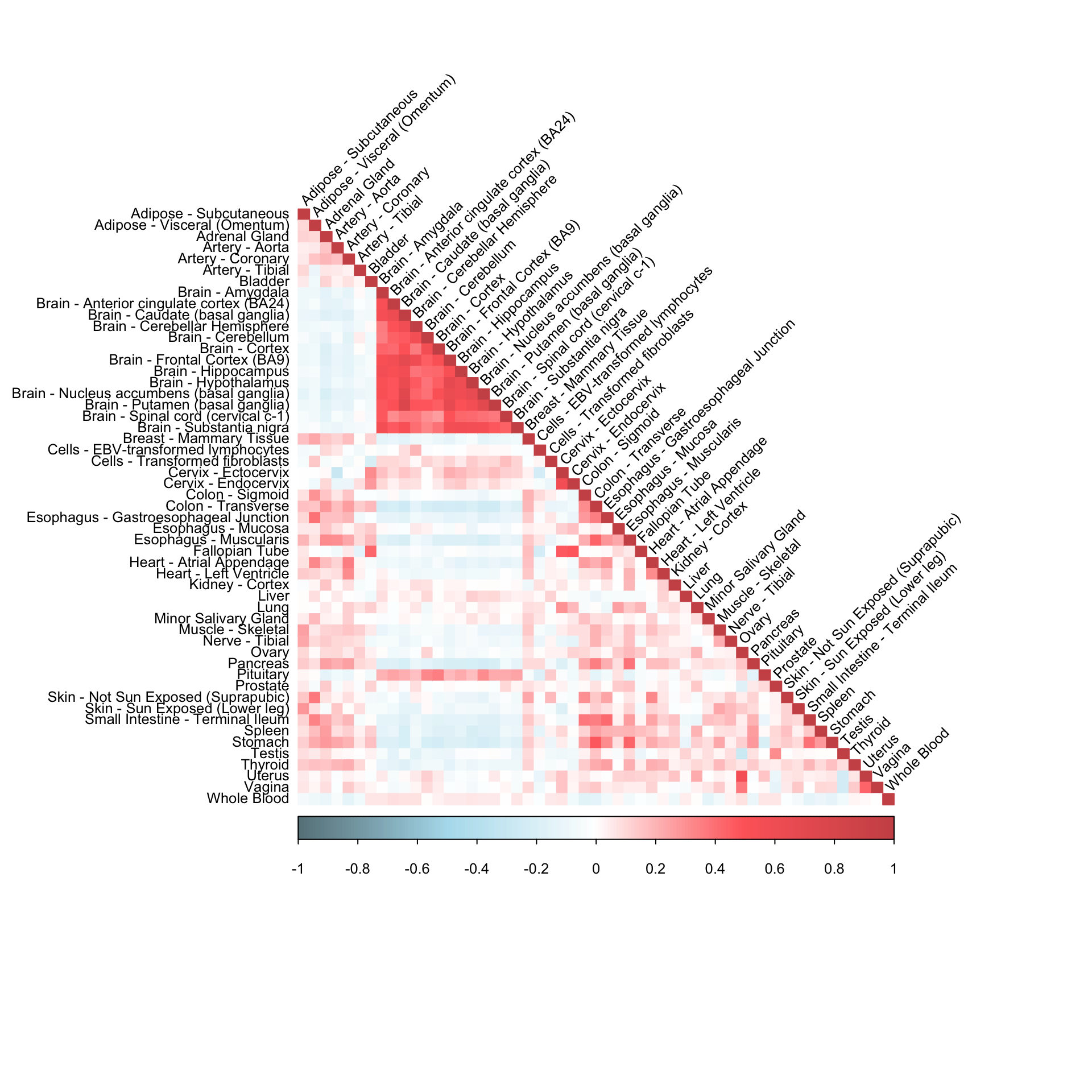
Pairwise sample correlation matrix
cormat = cor(gene_dat, use = "pairwise.complete.obs")
corrplot(cormat,   diag = TRUE,
         col = colorRampPalette(c("lightblue4", "lightblue2", "white", "indianred1", "indianred3"))(200),
         tl.pos = "ld", tl.cex = 0.8, tl.col = "black",
         rect.col = "white",na.label.col = "white",
         method = "color", type = "lower", tl.srt=45)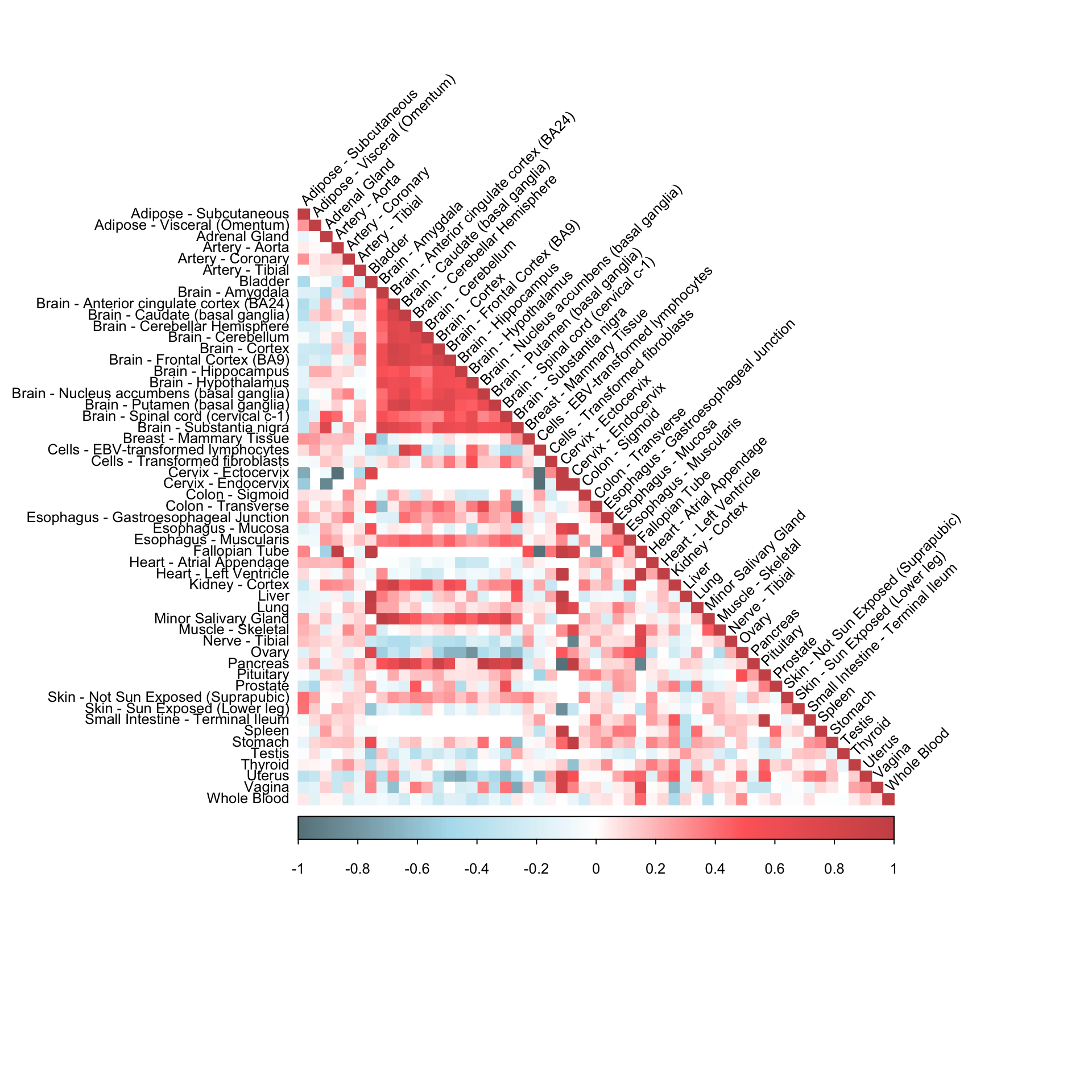
Session information
sessionInfo()R version 3.5.1 (2018-07-02)
Platform: x86_64-apple-darwin15.6.0 (64-bit)
Running under: macOS High Sierra 10.13.6
Matrix products: default
BLAS: /Library/Frameworks/R.framework/Versions/3.5/Resources/lib/libRblas.0.dylib
LAPACK: /Library/Frameworks/R.framework/Versions/3.5/Resources/lib/libRlapack.dylib
locale:
[1] en_US.UTF-8/en_US.UTF-8/en_US.UTF-8/C/en_US.UTF-8/en_US.UTF-8
attached base packages:
[1] stats graphics grDevices utils datasets methods base
other attached packages:
[1] softImpute_1.4 Matrix_1.2-14 corrplot_0.84 ggplot2_3.1.1
loaded via a namespace (and not attached):
[1] Rcpp_1.0.1 compiler_3.5.1 pillar_1.3.1
[4] git2r_0.23.0 plyr_1.8.4 workflowr_1.1.1
[7] R.methodsS3_1.7.1 R.utils_2.7.0 tools_3.5.1
[10] digest_0.6.19 lattice_0.20-35 evaluate_0.12
[13] tibble_2.1.1 gtable_0.3.0 pkgconfig_2.0.2
[16] rlang_0.4.2 yaml_2.2.0 withr_2.1.2
[19] stringr_1.4.0 dplyr_0.8.0.1 knitr_1.20
[22] rprojroot_1.3-2 grid_3.5.1 tidyselect_0.2.5
[25] glue_1.3.1 R6_2.4.0 rmarkdown_1.10
[28] purrr_0.3.2 magrittr_1.5 whisker_0.3-2
[31] backports_1.1.4 scales_1.0.0 htmltools_0.3.6
[34] assertthat_0.2.1 colorspace_1.4-1 stringi_1.4.3
[37] lazyeval_0.2.2 munsell_0.5.0 crayon_1.3.4
[40] R.oo_1.22.0 This reproducible R Markdown analysis was created with workflowr 1.1.1